Chapter 2 A Bifurcation Theorem for Resident-Invader Type Population

1. Introduction

In the field of population ecology, one major area to investigate is the requirement for species to persist and become extinct, and in epidemiology, one area of interest is both epidemics, sudden outbreaks of disease, and endemic situations. In this context, it is important to understand how external factors influence the dynamics of interacting populations or disease dynamics, and how they shape the long-term outcomes for both resident and invader populations. To study this, a bifurcation parameter is often varied to see when survival, extinction, or coexistence occurs. We use a bifurcation approach to discrete-time matrix models for invasion analysis.

We begin this chapter by extending the bifurcation theory presented in [Meissen2017Auth] to introduce the concept of invasion analysis in the context of interacting species such as host-paarsitoid type and epidemic dynamics. We then present the simplest discrete-time susceptible, infected, and recovered population model in epidemiology and discuss the global stability of the extinction equilibrium and the local stability of disease-free two-cycles. We further use the bifurcation theorem to analyze the stability of endemic dynamics.

2. Bifurcation Analysis of a Resident-Invader System of Host-Parasitoid Type

To study the interior dynamics of the matrix model, we apply a variation of the Fundamental Bifurcation Theorem, which describes the behavior of the nonlinear matrix equation

$$z(t+1)=A(z(t))z(t),$$

when a boundary $\theta$ periodic cycle for $\theta \ge 1$ destabilizes ([ackleh2023interplay, cushing1998introduction, elaydi2025discrete]). While classically used to study the persistence or extinction of a single (structured) species, this theorem has been extended to a number of other applications including evolutionary matrix models with multiple evolving traits ([cushing2017bifurcation]), competition ([Meissen2017Auth]), host-parasitoid systems ([ackleh2023interplay]), and epidemic models ([elaydi2025discrete]). In this chapter, we extend the results obtained in [Meissen2017Auth] to derive a general bifurcation result for a resident-invader system of host-parasitoid type. Here the key distinction between this model form and the competition form studied in ([Meissen2017Auth]) is that new invader individuals may be proportional to the number of resident individuals.

We consider a resident-invader system, consisting of a resident population with $m$ stages and an invader population with $n$ stages, given by the following equations:

(1)

where

$$x(t)={(x_1(t),x_2(t),\mathrm{\dots },x_m(t))}^T\in {ℝ}_{+}^m,$$

and

$$y(t)={(y_1(t),y_2(t),\mathrm{\dots },y_n(t))}^T\in {ℝ}_{+}^n,$$

represent the population sizes (or densities) in the resident and invader compartments, respectively. Here, we define $ℱ={({ℱ}_1,{ℱ}_2,\mathrm{\dots },{ℱ}_n)}^T$ and $𝒯={(T_1,T_2,\mathrm{\dots },T_n)}^T$ where for each $i\in 1,2,\mathrm{\dots },n$, ${ℱ}_i$ represents the number of new invaders that appear in compartment $i$ and ${𝒯}_i$ represents the number of individuals that transition to compartment $i$ from other invaders compartments. Similarly, we define $𝒢={(G_1,G_2,\mathrm{\dots },G_m)}^T$ where for each $i\in 1,2,\mathrm{\dots },m$, ${𝒢}_i$ represents the number of individuals in the resident compartment $i$.

We assume that the resident has a stable $\theta$ periodic cycle for $\theta \ge 1$. To study the invasion of another species into the resident system, we introduce a bifurcation parameter $\beta$ and write the system (1) as the following matrix model equation:

(2) $X(t+1)=P(\beta ,X)X(t),$

where $X(t)=(x(t),y(t))\in {ℝ}_{+}^{m+n}$ and $P(\beta ,X)$ is the projection matrix for system (1) given as,

(3)

Here, the matrices $P_{xx}(\beta ,X)\in {ℝ}^{m\times m}$ and $P_{xy}(\beta ,X)\in {ℝ}^{m\times n}$ determine the contribution of resident and invader individuals, respectively, to the resident stages while the matrices $P_{yx}(\beta ,X)\in {ℝ}^{n\times m}$, $P_{yy}(\beta ,X)\in {ℝ}^{n\times n}$ determine the contributions of resident and invader individuals, respectively, to the invader stages. We require the entries of the projection matrix to be non-negative and sufficiently smooth for calculation. Specifically, we assume

Assumption A1: The entries of $P$ defined in (3) are in $C^2(\mathrm{\Gamma },\mathrm{\Omega })$, where $\mathrm{\Gamma }\subset ℝ$ is an open interval and $\mathrm{\Omega }\supset {ℝ}_{+}^{m+n}$ is an open set, and are non-negative for $\beta \in \mathrm{\Gamma }$ and $x\in {ℝ}_{+}^{m+n}$.

We assume that system (2) has an invader-free non-trivial resident cycle of period $\theta \ge 1$ which we denote by $\tau =col({\tau }_x,0_{1\times n})$. That is, $\tau$ is a resident-only fixed point of the $\theta$ composite system,

$$X(t+1)=P^{(\theta )}(\beta ,X(t))X(t).$$

The $\theta$ composite Jacobian matrix of system (2) evaluated at $\tau$ has the form,

where $J_{xx}^{(\theta )}(\beta ,\tau )\in {ℝ}^{m\times m}$ and $J_{yy}^{(\theta )}(\beta ,\tau )\in {ℝ}^{n\times n}$. We further assume that the stability of this resident-only cycle is determined by the resident equations. Namely:

Assumption A2: $J_{yx}^{(\theta )}(\beta ,\tau )=0$ and the absolute value of the dominant eigenvalue of $J_{xx}^{(\theta )}(\beta ,\tau )$ is less than one for all $\beta$.

We consider what happens when an invader is introduced, destabilizing the resident cycle. Specifically, we assume

Assumption A3: The matrix $J_{yy}^{(\theta )}(\beta ,\tau )$ is non-negative and primitive. There exists a ${\beta }^0\in \mathrm{\Gamma }$ where the strictly dominant eigenvalue of $J_{yy}^{(\theta )}({\beta }^0,\tau )$ equals 1 and the corresponding right eigenvector $v_y$ and left eigenvector $w_y$ of $J_{yy}^{(\theta )}({\beta }_0,\tau )$ satisfy $w_y{\partial }_{\beta }^0{J}_{yy}^{(\theta )}{v}_x\ne 0$, where the superscript 0 denotes the evaluation at the bifurcation point $({\beta }^0,\tau )$.

Remark 2.1.

In [Meissen2017Auth], Meissen considered a general form of resident-invader interactions that encompasses cases such as competing species or predator-prey interactions. For these types of interactions, it is assumed that $P_{xy}(\beta ,X)$ and $P_{yx}(\beta ,X)$ are zero, meaning that individuals of type $y$ cannot arise from individuals of type $x$, and vice versa. In [ackleh2023interplay], the authors extended these results to host-parasitoid type interactions, allowing for $P_{yx}(\beta ,X)$ to be non-zero. Biologically, this term represents the creation of new parasitoids from hosts. Epidemic models share a similar structure to host-parasitoid systems except that $P_{xy}(\beta ,X)$ may also be non-zero, typically representing recovery from the disease. Moreover, for generality, here we allow all submatrices to depend on $\beta$, which also does not affect the results.

Theorem 1 establishes the direction of bifurcation and stability of the branch of $\theta$-cycles that bifurcate from the resident-only cycle at ${\beta }^0$. This analysis closely follows that presented in [Meissen2017Auth] (Specifically, the proof of Theorem 5 in [Meissen2017Auth]).

Theorem 1.

There exists a branch of solutions of the form

(4)

bifurcating from the resident-only cycle $(\beta ,\tau )$ of system (2) at $\beta ={\beta }^0$. The bifurcation is forward if $\kappa >0$ and backward if , where

(5) $$\kappa :=-\frac{w_y{D}_3(v)v_x+w_y{D}_4(v)v_x}{w_y{\partial }_{\beta }^0{J}_{yy}^{(\theta )}{v}_y}.$$

Near the bifurcation point $({\beta }^0,\tau )$, the cycle is asymptotically stable if and unstable if ${\lambda }_1>0$, where

(6) $${\lambda }_1:=\frac{w_y{D}_3(v)v_x+w_y{D}_4(v)v_x}{w_y{v}_x}.$$

Here

$$v:=col(v_x{v}_y)w:=(0_{1\times m}{w}_y),$$

denote the right and left eigenvectors, respectively, of $J_0^{(\theta )}=J^{(\theta )}({\beta }^0,\tau )$ corresponding to the eigenvalue 1, and $D_3(v_y)$ and $D_4(v_y)$ denote the bottom left $n\times m$ block and bottom right $n\times n$ block, respectively, of the matrix $D(v)$, where $d_{ij}(v):={\nabla }_X^0{p}_{ij}.v$.

Proof.

The Jacobian matrix of the $\theta$ composite system evaluated at $\tau$ can be written as,

(7) $J^{(\theta )}(\beta ,\tau )=P^{(\theta )}(\beta ,\tau )+{\displaystyle \sum _{k=1}^{m+n}}{\tau }_k{\partial }_{x_j}^0{P}_{ik}^{(\theta )}.$

The right eigenvector of $J^{(\theta )}({\beta }^0,\tau )$ corresponding to the eigenvalue 1 has the form

$$v=\left(\begin{array}{c}{v}_x\\ v_y\end{array}\right),$$

where the $m\times 1$ vector $v_x$ may be negative but the $n\times 1$ vector $v_y$ is the positive eigenvector of $J_{yy}^{(\theta )}({\beta }^0,\tau )$ corresponding to the eigenvalue 1 which is guaranteed by the Perron Frobenius Theorem, i.e. $v_y>0$, where $J_{yy}^{(\theta )}({\beta }^0,\tau )v_y=v_y$. The left eigenvector is

where the $1\times n$ vector $w_y$ is the positive left eigenvector of $J_{yy}^{(\theta )}({\beta }^0,\tau )$ corresponding to the eigenvalue 1, i.e, $w_y>0$, where $w_y{J}_{yy}^{(\theta )}({\beta }^0,\tau )=w_y$.

By Assumption A2 and A3, the strictly dominant eigenvalue of $J_{yy}^{(\theta )}({\beta }^0,\tau )$ is also the dominant eigenvalue of $J^{(\theta )}({\beta }^0,\tau )$. At ${\beta }^0$, ${(J_I^I)}^{(\theta )}({\beta }^0,\tau )$, and hence $J^{(\theta )}({\beta }^0,\tau )$ has simple dominant eigenvalue of 1. If $w{\partial }_{\beta }^0{J}^{(\theta )}v\ne 0$, then by the Lyapunov- Schimit Reduction which utilizes the Implicit function Theorem and the Fredholm Alternative, we obtain a branch of solutions of (2) which bifurcates from $({\beta }^0,\tau )$, given by

(8) $$\beta (ϵ)={\beta }^0+\kappa ϵ+o(ϵ),x(ϵ)=\tau +vϵ+u{ϵ}^2+o({ϵ}^2).$$

Since $v_y\in {ℝ}_{+}^n$, this branch exists for $ϵ>0$. Therefore, indicates a forward (backward) bifurcation. To determine the direction of bifurcation, we parameterize the variables in $ϵ$ along the branch of bifurcating fixed points of the $\theta$ composite system. These expansions include the state variable $x(ϵ)$, the bifurcation parameter $\beta (ϵ)$ as given above, the Jacobian $J^{(\theta )}(\beta (ϵ),x(ϵ))$ and the eigenvalue $\lambda (ϵ)$,

(9) $\lambda (ϵ)=1+{\lambda }_1ϵ+o(ϵ),$

$J^{\theta }(\beta (ϵ),x(ϵ))=J_0^{\theta }+J_1^{\theta }ϵ+o(ϵ).$

The expansion of $\beta (ϵ),x(ϵ)$ are determined by Theorem 1, the eigenvalue expansion guaranteed by Theorem 2 in [Meissen2017Auth] and the expansion of $J(\beta (ϵ),x(ϵ))$ guaranteed by the smoothness provided by Assumption A1.

To derive a formula for $\kappa$, we Taylor expand the $\theta$ composite map and substitute the expansion of $x(ϵ)$ and $\beta (ϵ)$ into the Taylor expansion and equate orders of $ϵ.$ We first compute the Taylor expansion of the right-hand side of $x_i={\sum }_j{x}_j{P}_{ij}^{(\theta )}(\beta ,x)$ in terms of $x$ and $\beta$ near $({\beta }^0,\tau )$. Recall the superscript $0$ denotes evaluation at $({\beta }^0,\tau ).$ By the Taylor expansion we have,

$x_i=$ ${\tau }_i+(\beta -{\beta }^0){\displaystyle \sum _j}{\tau }_j{(p_{ij}^{(\theta )})}_{\beta }^0+{\displaystyle \sum _j}(x_j-{\tau }_j)\left[{(p_{ij}^{(\theta )})}^0+{\displaystyle \sum _k}{\tau }_k{(p_{ik}^{(\theta )})}_{x_j}^0\right]$

$+{\displaystyle \frac{1}{2}}{(\beta -{\beta }^0)}^2{\displaystyle \sum _j}{\tau }_j{(p_{ij}^{(\theta )})}_{\beta \beta }^0+(\beta -{\beta }^0){\displaystyle \sum _j}(x_j-{\tau }_j)\left[{(p_{ij}^{(\theta )})}_{\beta }^0+{\displaystyle \sum _k}{\tau }_k{(p_{ik}^{(\theta )})}_{\beta x_j}^0\right]$

$+{\displaystyle \frac{1}{2}}{\displaystyle \sum _j}(x_j-{\tau }_j){\displaystyle \sum _k}(x_k-{\tau }_k)\left[2{(p_{ik}^{(\theta )})}_{\beta }^0+{\displaystyle \sum _r}{\tau }_k{(p_{ir}^{(\theta )})}_{x_k{x}_j}^0\right]+o_2,$

were $o_2$ contains all terms of a higher order than two in combination of $x$ and $\beta -{\beta }^0.$ Terms 2 and 4 on the right-hand side evaluate to zero due to the structure of $0$’s in $\tau =col({\tau }_r,0_{n\times 1})$ and $P^{(\theta )}(\beta ,\tau ).$ Next, we substitute the expansion of $x(ϵ)$ and $\beta (ϵ)$ from (8) into the Taylor expansion and equate the order of $ϵ$.
At order ${ϵ}^0$, we see that, ${\tau }_i={\tau }_i$.
At order ${ϵ}^1$, we see that,

$$v_i=\sum _j{v}_j\left[{(p_{ij}^{(\theta )})}^0+\sum _k{\tau }_k{(p_{ik}^{(\theta )})}_{x_j}^0\right]={(P^{(\theta )}({\beta }^0,\tau )v)}_i+\sum _j{v}_j\sum _k{\tau }_k{(p_{ik}^{(\theta )})}_{x_j}^0.$$

At order ${ϵ}^2$, we see

$u_i$ $={\displaystyle \sum _j}{u}_j\left[{(p_{ij}^{(\theta )})}^0+{\displaystyle \sum _k}{\tau }_k{(p_{ik}^{(\theta )})}_{x_j}^0\right]+k{\displaystyle \sum _j}{v}_j\left[{(p_{ij}^{(\theta )})}_{\beta }^0+{\displaystyle \sum _k}{\tau }_k{(p_{ik}^{(\theta )})}_{\beta x_j}\right]+$

$+{\displaystyle \frac{1}{2}}{\displaystyle \sum _j}{v}_j{\displaystyle \sum _k}{v}_k\left[2{(p_{ik}^{(\theta )})}_{xj}^0+{\displaystyle \sum _r}{\tau }_r{(p_{ir})}_{x_k{x}_j}^0\right]$

$={(J_0^{(\theta )}u)}_i+k{({\partial }_{\beta }^0{J}^{(\theta )}v)}_i+{\displaystyle \sum _j}{v}_j({\nabla }_x^0{p}_{ij}^{(\theta )}.v)+{\displaystyle \frac{1}{2}}{\displaystyle \sum _j}{v}_j{\displaystyle \sum _k}{v}_k\left[{\displaystyle \sum _r}{\tau }_r{(p_{ir}^{(\theta )})}_{x_k{x}_j}^0\right].$

We denote this as

$$u=J_0^{(\theta )}u+k{\partial }_{\beta }^0{J}^{(\theta )}v+D(v)v+H(v)v,$$

where $d_{ij}(v)={\nabla }_x^0{p}_{ij}^{(\theta )}\cdot v$ and $h_{ij}(v)=\frac{1}{2}{\sum }_k{v}_k\left[{\sum }_r{\tau }_r{(p_{ir}^{(\theta )})}_{x_k{x}_j}^0\right].$
By the Fredholm Alternative,

$$(I-J_0^{(\theta )})u=\kappa {\partial }_{\beta }^0{J}^{(\theta )}v+D(v)v+H(v)v,$$

is solvable for $u$ if and only if

$$w(\kappa {\partial }_{\beta }^0{J}^{(\theta )}v+D(v)v+H(v)v)=0,$$

The structure of

$$H\left(v\right)=\left(\begin{array}{c}{\star }_{m\times \left(m+n\right)}\\ 0_{n\times \left(m+n\right)}\end{array}\right),$$

along with of results in $wH(v)v=0$. Solving for $\kappa$ we find,

$$\kappa =-\frac{wD(v)v}{w{\partial }_{\beta }^0{J}^{(\theta )}v}.$$

We use $w{\partial }_{\beta }^0{J}^{(\theta )}v=w_I{\partial }_{\beta }^0{(J_I^I)}^{(\theta )}{v}_I$ to simplify the denominator. To simplify the numerator, note that the form means that only the bottom left $n\times m$ and bottom right $n\times m$ blocks of $D(v)$ denoted $D_3$ and $D_4$ respectively, effect $\kappa$. If the bifurcation parameter is strictly beneficial to the invader (i.e., if $\beta$ represents the reproduction rate), the entries of ${\partial }_{\beta }^0{(J_I^I)}^{(\theta )}$ are positive. Therefore, the direction of the bifurcation is determined by the numerator of $\kappa .$

Finally we calculate ${\lambda }_1$ to determine the stability of the $\theta$ cycles bifurcating from $({\beta }^0,\tau )$. Notice that, if cycles are stable and if ${\lambda }_1>0$ cycles are unstable. Let

$$\xi (ϵ)=v+{\xi }_1ϵ+o(ϵ),$$

denote the eigenvector of $J^{(\theta )}(ϵ)=J^{(\theta )}(\beta (ϵ),x(ϵ))$ corresponding to $\lambda (ϵ)$. The eigenvalue equation and its differential with respect to $ϵ$ give us,

$$J^{(\theta )}(ϵ)\xi (ϵ)=\lambda (ϵ)\xi (ϵ),$$

$${(J^{(\theta )})}^{\prime }(ϵ)\xi (ϵ)+J^{(\theta )}(ϵ){\xi }^{\prime }(ϵ)={\lambda }^{\prime }(ϵ)\xi (ϵ)+\lambda (ϵ){\xi }^{\prime }(ϵ).$$

At $ϵ=0$, these reduce to

$$J_0^{(\theta )}v=v,$$

$$J_1^{(\theta )}v+J_0^{(\theta )}{\xi }_1={\lambda }_{1}v+{\xi }_1.$$

The first equation holds because $v$ is a right eigenvector of $J_0^{(\theta )}$ corresponding to eigenvalue 1. The second equation is equivalent to

$$(J_0^{(\theta )}-I)\xi ={\lambda }_{1}v-J_1^{(\theta )}v.$$

By the Fredholm Alternative, it is solvable if and only if

$$w({\lambda }_{1}v-J_1^{(\theta )}v)=0.$$

Thus,

(10) ${\lambda }_1={\displaystyle \frac{w{J}_1^{(\theta )}v}{wv}}.$

We then compute $J_1^{(\theta )}$ using

${(J_1^{(\theta )})}_{ij}$ $={{\displaystyle \frac{d}{dϵ}}\left[p_{ij}^{(\theta )}+{\displaystyle \sum _k}{x}_k{\partial }_{x_j}{p}_{ik}^{(\theta )}\right]|}_{ϵ=0}$

$=\left[{(p_{ij}^{(\theta )})}_{\beta }^0+{\displaystyle \sum _k}{\tau }_k{\partial }_{x_j}{(p_{ik}^{(\theta )})}_{\beta x_j}^0\right]\kappa$

$+{\displaystyle \sum _k}{v}_k{(p_{ij}^{(\theta )})}_{x_k}^0+{\displaystyle \sum _k}{v}_k{(p_{ik}^{(\theta )})}_{x_j}^0$

$+{\displaystyle \sum _r}{v}_r{\displaystyle \sum _k}{\tau }_k{(p_{ik}^{(\theta )})}_{x_j{x}_r}^0.$

Now letting $g_{ij}(v)={\sum }_k{v}_k{(p_{ik}^{(\theta )})}_{x_j}^0$, we can write this as

$$J_1^{(\theta )}=\kappa {\partial }_{\beta }^0{J}^{(\theta )}+D(v)+G(v)+2H(v),$$

Note that,

and recall that $wH(v)v=0$, so that (10) gives,

${\lambda }_{1}wv=$ $w{J}_1^{(\theta )}v,$

$=$ $w(\kappa {\partial }_{\beta }^0{J}^{(\theta )}+D(v)+G(v)+2H(v))v,$

$=$ $w(\kappa {\partial }_{\beta }^0{J}^{(\theta )}+2D(v))v,$

$=$ $\kappa w{\partial }_{\beta }^0{J}^{(\theta )}v-2\kappa w{\partial }_{\beta }^0{J}^{(\theta )}v,$

$=$ $-\kappa w{\partial }_{\beta }^0{J}^{(\theta )}v.$

which results in ${\lambda }_1$ being given by Equation (6). ∎

3. An SIR Model with Demographic Population Cycles

We now illustrate the application of Theorem 1 to simple SIR model. Let $S(t)$, $I(t)$, $R(t)$ denotes the susceptible, infectious (infected with the disease), and recovered population densities at time $t\in \{0,1,2,\mathrm{\dots }\}$, and $N(t)=S(t)+I(t)+R(t)$ represents the total population. To introduce a SIR model with periodic demography, we first assume that a susceptible individual $S(t)$ can be infectious and that an infectious individual $I(t)$ can recover from the infection at each time unit. We assume that susceptible individuals have to be in the infectious class before recovering. Individuals in the recovered class $R(t)$ are neither susceptible nor infectious and thus acquire lifelong immunity. This means that once the individuals are in the recovered class, they never get infected again. We also assume the susceptible population who interact with the infectious population become infectious with probability $(1-\varphi (I(t)))$ and escape infection with probability $\varphi (I(t))$ at each time unit. Furthermore, we assume that infectious individuals recover from the infection with constant probability $\gamma \in (0,1)$ and remain infectious with constant probability $(1-\gamma )$ at each time unit. We assume that the probability of natural death is $d\in (0,1)$ each time unit.

Following [yakubu2010introduction], the escape’ function

$$\varphi :[0,\mathrm{\infty })\to [0,1],$$

is assumed to be a nonlinear, decreasing, smooth, concave up function with $\varphi (0)=1$. That is and ${\varphi }^{\prime \prime }(x)>0$ for all $x\ge 0.$ For example, when infections are modeled as a Poisson process, then $\varphi (I(t))=\exp (-\beta I(t))$ with the transmission constant $\beta >0$.

To include the demography, we let

$$g:[0,\mathrm{\infty })\to [0,\mathrm{\infty }),$$

denote the recruitment (birth or immigration) function of individuals to the susceptible class per unit of time, where $g(0)=\underset{t\to \mathrm{\infty }}{lim}g(N(t))=0$. A classic example of the recruitment function is the Ricker recruitment function,

$$g(N(t))=rN(t){\exp }^{-bN(t)},$$

where the intrinsic growth rate $r>0$ and the scaling parameter $b>0.$

In model (11), we assume the order of events happens in the following order: disease transmission and recovery, survival (death), and reproduction. However, in real biological systems, these events may happen in different orders. Based on these assumptions, the discrete-time SIR model takes the following form:

(11)

where, $x=(S,R)$ and $y=I$ is the non-infectious and infectious individuals respectively. In model (11) the total population size is given by $N(t)=g(N(t))+(1-d)N(t)$.

Given the assumptions on $g(N(t))$ that . Hence,

(12) $$N(t+1)\le D+(1-d)N(t).$$

It follows that,

$$\underset{t\to \mathrm{\infty }}{lim\; sup}N(t)\le \frac{D}{d}=:\widehat{N}.$$

Thus for any $\eta >0$, there exists a $T>0$, which depends on $S(0),I(0),V(0)$ such that for $t>T$, $N(t)\le \widehat{N}(1+\eta ).$ Hence, for any $\eta >0$, every forward solution of (12) enters the positively invariant set

(13) $$\{(S,I,R)\in {ℝ}_{+}^3|S+I+R\le \widehat{N}(1+\eta )\}$$

in finite time.

We make the assumption that total population $N(t)$ in model (11) tends to a positive constant, denoted by $N_{\mathrm{\infty }},$ as $t\to \mathrm{\infty }.$ Hence, by the limiting asymptotic theory ([zhao2003dynamical]) the model reduces to the following system:

(14)

We assume, The model (14) has unique disease free equilibrium $(\tau ,0,0)=(N_{\mathrm{\infty }},0,0)$ and we study the global stability of it. In addition, we assume that linearization of model (11) about the disease-free equilibrium $(\tau ,0,0)$ yeilds the linearized system

$$Z(t+1)=J(\tau ,0,0)Z(t),$$

where $Z(t)=(S(t),I(t),R(t))\in {ℝ}_{+}^3$. Following [van2019disease], To compute $R_0$ by the next generation matrix approach, we have,

$$ℱ=(1-d)S(t)(1-\varphi (I(t)))\text{and}𝒯=(1-d)(1-\gamma )I(t),$$

from which we have,

$$F=-(1-d)\tau {\varphi }^{\prime }(0),\text{and}T=(1-d)(1-\gamma ),$$

where $F$ is the matrix of new infections that survive the time interval, and $T$ is the transition matrix. Hence, the basic reproduction number,

(15) $$R_0=\frac{-(1-d)\tau {\varphi }^{\prime }(0)}{1-(1-d)(1-\gamma )}.$$

In the following theorem, we discuss the global stability of the disease-free equilibrium and the stability of the endemic equilibrium bifurcating from it.

Theorem 2.

Consider the SIR model (11)

1. The disease free equilibrium $(\overline{S},0,0)=(\tau ,0,0)$, where $\tau =N_{\mathrm{\infty }}$. It is locally asymptotically stable if and unstable if $R_0>1$. Furthermore, the disease-free equilibrium is globally asymptotically stable if , where $R_0$ is defined in (15).

2. At $R_0=1$, there exists a branch of endemic equilibria bifurcating from the disease-free equilibrium. The bifurcation is forward (supercritical), and the equilibria are locally asymptotically stable for $R_0⪆1$.

Proof.

(a) Following the next generation matrix method in [allen2008basic], we know that the DFE is locally asymptotically stable if and unstable if $R_0>1.$ Next, we discuss the global stability of the disease-free equilibrium when . We apply Theorem 3 from [van2019disease], which establishes the global stability of the disease-free equilibrium for a general class of discrete-time epidemic models using the Lyapunov function

$$L(y(t))=\omega {(I-T)}^{-1}y(t),$$

where $y$ is the vector of infectious compartments, $I$ denotes the identity matrix, and $\omega >0$ is the left eigenvector of ${(I-T)}^{-1}F$. To apply this theorem, the following conditions must hold:

• and ${(I-I)}^{-1}F$ is irreducible.

• There is a compact forward invariant set $\overline{\mathrm{\Omega }}\subset {ℝ}_{+}^{m+n}$ containing the unique disease-free equilibrium $(\overline{x},0)$ such $f(\overline{x},0)=0$ and $f(x(t),y(t))\ge 0$ for all $(x(t),y(t))$ in $\overline{\mathrm{\Omega }}$ where

  $f(x(t),y(t)):=$ $(F+T)y(t)-(ℱ(x(t),y(t))+𝒯(x(t),y(t))).$

It is easy to verify that the conditions in (i) are satisfied as well as $f(\overline{x},0)=0$. It remains to check the non-negativity condition $f(x(t),y(t))\ge 0$. We have,

$$S(t+1)\le g(N_{\mathrm{\infty }})+(1-d)S(t)$$

Since, ${lim}_{t\to \mathrm{\infty }}S(t)=N_{\mathrm{\infty }}$, there exists a $T>0$ and $\eta >0$ such that $S(t)\le \overline{S}(1+\eta ).$ Then we may consider the compact forward invariant set $\overline{\mathrm{\Omega }}:=[0,\overline{S}(1+\eta )]\times [0,\widehat{N}(1+\eta )]\times [0,\widehat{N}(1+\eta )]$. Therefore,

(16) $$f(x(t),y(t))=(1-d)[-\overline{S}{\varphi }^{\prime }(0)I(t)-S(t)(1-\varphi (I(t)))]$$

By the Mean Value Theorem, we have,

$$-{\varphi }^{\prime }(0)I(t)>1-\varphi (I(t))\ge 0.$$

we may choose $\eta$ sufficiently small so that

$$-\overline{S}{\varphi }^{\prime }(0)I(t)>S(t)(1+\eta )(1-\varphi (I(t)))\ge S(t)(1-\varphi (I(t))).$$

Hence,

$$f(x(t),y(t))\ge 0$$

for all $x(t),y(t)\in \widehat{\mathrm{\Omega }}.$ Then the global stability of the disease-free equilibrium follows from Theorem 3 in [van2019disease].
(b) We consider $x=(S,R)$ and $y=I$ as the non disease and disease compartments. The projection matrix of system (11) is,

(17)

Let $\tau$ denote the disease-free equilibrium $(\tau ,0,0)$ and ${\beta }^0$ be defined such that $R_0=1$. The Jacobian evaluated at $({\beta }^0,\tau )$ is,

The Jacobian matrix has a simple eigenvalue 1 at $\beta ={\beta }^0$ with corresponding right eigenvector

where,

$v_1:=$ $-{\displaystyle \frac{\tau {\varphi }^{\prime }(0)}{\gamma +\tau {\varphi }^{\prime }(0)}},$

$v_2:=$ $-{\displaystyle \frac{\gamma }{\gamma +\tau {\varphi }^{\prime }(0)}},$

and left eigenvector

Next, to determine the direction of bifurcation $\kappa$ and stability of the bifurcating equilibria, as determined by ${\lambda }_1$, as given in Theorem 1 we calculate,

$$D_3(v_y)=-(1-d){({\varphi }^{\prime })}^0(\beta ,0),\text{and}{\partial }_{\beta }^0{J}_y^y=-(1-d)\tau {({\varphi }^{\prime })}_{\beta }^0(\beta ,0).$$

Thus we obtain,

$$\kappa =-\frac{{({\varphi }^{\prime })}^0(\beta ,0)v_1}{\tau {({\varphi }_{\beta }^{\prime })}^0(\beta ,0)},\text{and}{\lambda }_1=-(1-d){({\varphi }^{\prime })}^0(\beta ,0)v_1.$$

We find for $R_0=1$. As a result, $\kappa >0$ and . Thus, it follows that at $({\beta }_2^0,\tau )$ there exists a forward bifurcating branch of stable endemic equilibrium. ∎

Next, we consider the case where disease-free state is stable two cycle. We examine what happens when disease invade. We show that when $R_0⪆1$ a branch of endemic two cycle are bifurcating from the disease-free two cycle and are locally asymptotically stable. Particularly, we assume that the model (14) has a unique disease-free two-cycle ${\tau }_c$, where ${\tau }_c=\{{\tau }_1,{\tau }_2\}$ and we study the stability of disease-free two cycle ${\tau }_c$ and a branch of endemic period two cycle bifurcating from it. To study the stability of the disease-free period two population cycle $({\tau }_c,0,0)$ of model (11), we calculate $R_0^c$ for the model (11) with demographic-period population. To compute the basic reproduction number, $R_0^c$ for model (11), from [van2019demographic], by the next generation matrix method, for each $j\in \{1,2\}$,

$$F_j=[-(1-d)z_j{\varphi }^{\prime }(0)]\text{and}{T}_j=[(1-d)(1-\gamma )],$$

The transition matrix is,

$$T={((1-d)(1-\gamma ))}^2,$$

and the matrix of new infections is

$F=$ $(F_2+T_2)(F_1+T_1)-T.$

$=$ ${(1-d)}^2\left[{\displaystyle \prod _{j=1}^2}\left(-z_j{\varphi }^{\prime }(0)+(1-\gamma )\right)-{(1-\gamma )}^2\right].$

Hence, the basic reproduction number is

(18) $$R_0^c=\rho (F{(I-T)}^{-1})=\frac{{(1-d)}^2\left[{\prod }_{j=1}^2\left(-z_j{\varphi }^{\prime }(0)+(1-\gamma )\right)-{(1-\gamma )}^2\right]}{1-{(1-d)}^2{(1-\gamma )}^2}.$$

Using this $R_0^c$, we say, the disease free period-two cycle $({\tau }_c,0,0)$ where ${\tau }_c=\{{\tau }_1,{\tau }_2\}$ of the model (11) is locally asymptotically stable if and unstable if $R_0^c>1.$ Proof of the statement follows from Theorem 2.1 in [allen2008basic] and is omitted. However, in Theorem 3 (cited in [elaydi2002global]), the authors showed that global stability of the disease-free period-two cycle is not possible in the autonomous discrete-time model (11).

In the next theorem, we prove the existence and stability of a branch of endemic two-cycle bifurcating from the stable disease-free two-cycle using the bifurcation theorem 1 presented in Chapter LABEL:chapter1.5.

Theorem 3.

Assume the model (11) has unique disease-free two cycle ${\tau }_c$. When $R_0^c=1$, there exists a branch of endemic two-cycle bifurcating from the disease-free two-cycle $({\tau }_c,0,0)$ of model (11). The bifurcation is forward (supercritical), and the equilibria are locally asymptotically stable for $R_0^c⪆1$.

Proof.

The projection matrix of the system (11) is defined in equation (17). Let ${\tau }_c$ denote the disease-free equilibria ${\tau }_c$ of the following two-composite system

$$X(t+1)=P^2(\beta ,X(t))X(t),$$

and ${\beta }^0$ be defined such that $R_0^c=1$. The composite Jacobian evaluated at $({\beta }^0,{\tau }_c)$ is,

The composite Jacobian matrix has a simple eigenvalue 1 at ${\beta }_2={\beta }_2^0$ with corresponding right eigenvector

where,

$v_1^{(2)}:=$ ${\displaystyle \frac{{\varphi }^{\prime }(\beta ,0)({\tau }_1+{\tau }_2(1-\gamma )-{\tau }_1{\tau }_2{\varphi }^{\prime }(\beta ,0))}{(\gamma -2)\gamma -({\tau }_1+{\tau }_2)(1-\gamma ){\varphi }^{\prime }(\beta ,0)+{\tau }_1{\tau }_2{({\varphi }^{\prime }(\beta ,0))}^2}},$

$v_2^{(2)}:=$ $-{\displaystyle \frac{\gamma (\gamma -2+{\tau }_1{\varphi }^{\prime }(\beta ,0))}{(\gamma -2)\gamma -({\tau }_1+{\tau }_2)(1-\gamma ){\varphi }^{\prime }(\beta ,0)+{\tau }_1{\tau }_2{({\varphi }^{\prime }(\beta ,0))}^2}},$

and left eigenvector

Next, to determine the direction of bifurcation $\kappa$ and stability of the bifurcating equilibria, as determined by ${\lambda }_1$, as given in Theorem 1, from

we find

$D_3^{(2)}(v^{(2)})=$ $-(1-d)(1-\gamma ){\varphi }^{\prime }(\beta ,0)$

$-(1-d)\left(1-d+{\displaystyle \frac{g(N_{\mathrm{\infty }})}{{\tau }_c}}\right){\varphi }^{\prime }(\beta ,0)$

$\times ((1-d)(1-\gamma )((1-d)(1-\gamma )-(1-d){\tau }_c{\varphi }^{\prime }(0))$

$-(1-d)((1-d){\tau }_c+g(N_{\mathrm{\infty }})){\varphi }^{\prime }(\beta ,0)((1-d)(1-\gamma )-(1-d){\tau }_c{\varphi }^{\prime }(\beta ,0))),$

which is positive, and from $J_{yy}^{(2)}(\beta ,x)$ we have ${\partial }_{\beta }^0{(J_{yy})}^{(2)},$ which is also positive. For large expressions, we omit their explicit form. Thus we obtain,

$${\kappa }^{(2)}=-\frac{D_{31}^2(v^{(2)}).v_1^{(2)}}{{\partial }_{\beta }^0{(J_{yy})}^{(2)}},$$

$${\lambda }_1^{(2)}=-{\kappa }^{(2)}{\partial }_{\beta }^0{(J_{yy})}^{(2)}.$$

We find for $R_0^c⪆1$. As a result, we have ${\kappa }^{(2)}>0$ and . Thus, it follows that at $({\beta }_2^0,\tau )$ there exists a forward bifurcating branch of a stable period two cycle for $R_0⪆1$. ∎

3.1. Numerical Examples

In this section, we show numerical examples to illustrate the results for model (11). For this, we use the Ricker recruitment function $g(N)=rN{e}^{-bN},$ where $r>0,b>0$ and the escape function $\varphi (I)=e^{-\beta I}$. For this choice of nonlinearities, when the total population converges to $N_{\mathrm{\infty }}=\frac{1}{b}\ln (\frac{r}{d})$, the disease free equilibrium $(\tau ,0,0)=(N_{\mathrm{\infty }},0,0)$, for any choice of parameters. The basic reproduction number is given by,

(19) $$R_0^c=\rho (F{(I-T)}^{-1})=\frac{{(1-d)}^c\left[{\prod }_{j=1}^c(z_j\beta +(1-\gamma ))-{(1-\gamma )}^c\right]}{1-{(1-d)}^c{(1-\gamma )}^c},$$

where $c$ represents period $c$ cycle ($c=1$ means an equilibrium and $c=2$ means a two cycle). For all simulations, we use the following parameter values:

(20) $$d=0.5,\gamma =0.5,b=0.1.$$

These parameters are from [van2019demographic]. In the following example, we show the local stability of the endemic equilibrium bifurcating from a stable disease-free equilibrium if $R_0⪆1.$

Example 3.1.

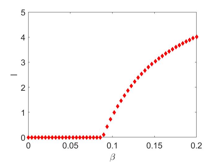
(Local stability of endemic equilibrium). In this example, we show the local stability of the endemic equilibrium of model (11). We use the force of infection of the invader, $\beta$, as the bifurcation parameter in this example. For the choice of non-linearities mentioned above, the critical value of the bifurcation parameter is

$${\beta }^0=\frac{1-(1-\gamma )(1-d)}{(1-d)\tau },$$

which is found by solving $R_0=1$ for $\beta$. The right eigenvector expression of the Jacobian matrix evaluated at the disease-free equilibrium is simplified to the following expression:

$$v_1=\frac{\tau {\beta }^0}{\gamma -\tau {\beta }^0},v_2=-\frac{\gamma }{\gamma -\tau {\beta }^0}.$$

It can be verified that and $v_2>0$, at $R_0=1$, we find,

$$D_3(v_y)=(1-d){\beta }^0,\text{and}{\partial }_{\beta }^0{J}_{yy}=(1-d)\tau .$$

Since these two expressions are positive, the sign of $v_1$ determines the direction and stability of the bifurcating equilibria:

To compare the numerical result for the stability of a branch of endemic equilibria obtained in [van2019demographic], with our analysis in Theorem (2), values given by (20), and the inherent infection growth rate $r=e^1$, we find the DFE, $\tau =16.9315$, and the critical value of the bifurcation ${\beta }^0=0.0886$ corresponding to the $R_0=1$. If we choose the force of infection $\beta =0.0986⪆{\beta }_0$, we find $R_0=1.11⪆1$ which implies . Finally, we have, $\kappa =5.9e^{-4}>0$ and for $R_0⪆1$ as proved in Theorem 2 (b). As a result, the model (11) exhibits forward bifurcation at $R_0=1$, corresponding to the $\beta =0.0886$.

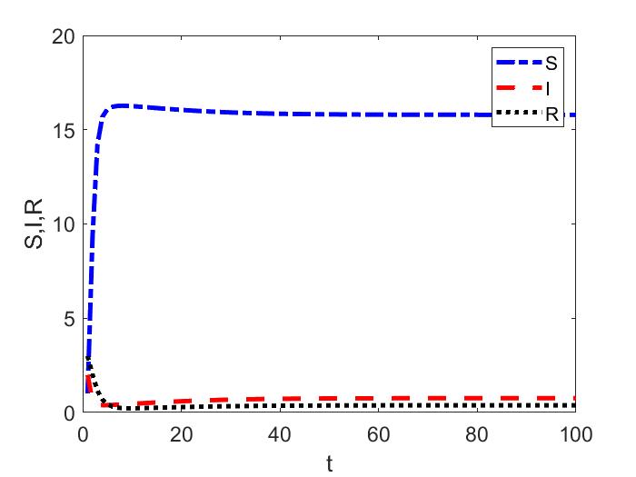
Hence, the endemic equilibria bifurcating from the disease-free equilibria are locally asymptotically stable when $R_0⪆1$ (Figure 1(a)). From the time series simulations we obtain the endemic equilibrium $(S^{\ast },I^{\ast },R^{\ast })=(15.79,0.76,0.38)$ for two different initial conditions close to each other (shown in Figure 1(b)).

(a)

(b)

Figure 1. (a) Shown is the bifurcation diagram for model (11) giving the asymptotic number of infected individuals using the parameter given in (20) and $r=e^1$. (b) Time series of $S(t),I(t),R(t)$ for model (11) with initial value $S(0)=1,I(0)=2,R(0)=3$. All graphs use the parameter values given in (20).

Since for the Ricker recruitment function, if $\frac{r}{d}>e^{\frac{2}{d}}$, then total population undergoes period doubling bifurcations ([elaydi2007discrete]). In the next example, we show the local stability of the a branch of endemic two-cycle bifurcating from the stable disease-free two-cycle.

Example 3.2.

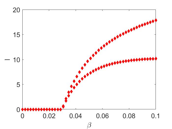
(Local stability of endemic two-cycle). In this example, we show the local stability of the endemic two-cycle bifurcating from the disease-free two-cycle of the model (11) when $1>\frac{r}{d}>e^{\frac{2}{d}}$. Specifically, using the Theorem 1, we show that at $R_0^{(2)}=1$, there is a branch of endemic two cycles from the stable disease-free two cycles, and the bifurcating two cycles are locally asymptotically stable if $R_0^{(2)}⪆1$. In [van2019demographic], using the parameters given in (20), authors showed numerically that the disease-free stable two cycles $({\tau }_1,{\tau }_2)=(37.883,65.757)$ when $r=e^4$ and four cycle at $({\tau }_1,{\tau }_2,{\tau }_3,{\tau }_4)=(41.473,85.957,44.560,73.743)$ when $r=e^{4.6}$. For the choice of parameter values given in (20) at ${\beta }^0=0.0299$ corresponding to the $R_0^{(2)}=1.$ The right eigenvector expression of the Jacobian matrix evaluated at the disease-free two cycles is simplified to the following expression:

$v_1^{(2)}=$ $-{\displaystyle \frac{{\beta }^0({\tau }_1+{\tau }_2(1-\gamma )+{\tau }_1{\tau }_2{\beta }^0)}{\gamma (\gamma -2)+({\tau }_1+{\tau }_2)(1-\gamma ){\beta }^0+{\tau }_1{\tau }_2{({\beta }^0)}^2}},$

$v_2^{(2)}=$ ${\displaystyle \frac{(2-\gamma +{\tau }_1{\beta }^0)\gamma }{\gamma (\gamma -2)+({\tau }_1+{\tau }_2)(1-\gamma ){\beta }^0+{\tau }_1{\tau }_2{({\beta }^0)}^2}}.$

It can be verified that and $v_2^{(2)}>0$ for $R_0^{(2)}=1$. We find,

$D_3^{(2)}(v_y)=$ $(1-d)(1-\gamma ){\beta }^0+{\beta }^0(1-d)\left((1-d)+{\displaystyle \frac{g(N_{\mathrm{\infty }})}{{\tau }_c}}\right)((1-d){\tau }_c{\beta }^0+(1-d)(1-\gamma )),$

which is clearly positive. We also find ${\partial }_{\beta }^0{J}_{yy}^{(2)}$ is always positive. Hence, ${\kappa }^{(2)}>0$ and . As a result, the model (11) demonstrates a forward bifurcating endemic two cycles at $R_0^{(2)}=1$, corresponding to the $\beta =0.03$ (see Figure (2(a))).

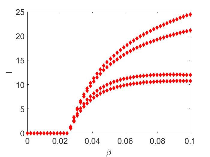
In Figure (2(a)), we are varying $\beta$ between $0$ to $0.1$, and we notice a bifurcating stable two-cycle. Keeping all the parameters the same as before, but if we increase $r$ from $e^4$ to $e^{4.6}$, numerically, we observe a locally asymptotically endemic stable four-cycle (Figure (2(b))) [not proved analytically].

(a)

(b)

Figure 2. Shown is the bifurcation diagram for model (11) giving the asymptotic number of infected individual. (a) Endemic-two cycle bifurcating from the disease-free two cycles as $R_0^{(2)}$ increases through 1 for model (11). The critical point of the bifurcation is ${\beta }_0=0.0299$. (b) Endemic-four cycle bifurcating from the disease-free four cycles as $R_0^{(2)}$ increases through 1 for model (11). For all the graphs, we use the parameters provided in (20).

4. Concluding Remarks

In this chapter, we have developed a framework for studying invasion analysis in a discrete-time structured population or epidemic model using an extension of the Fundamental Bifurcation Theorem. A main contribution of the chapter is the extension of a bifurcation theorem for resident-invader population presented in [Meissen2017Auth]. In particular, by allowing the off-diagonal blocks of the projection matrix to be nonzero, the formulation encompasses not only competition-type interactions but also host–parasitoid and epidemic-type interactions in which one population can generate individuals in the other (for example, new parasitoids produced through parasitized hosts, or recovery moving individuals from infected to recovered compartments). Under certain assumptions, the theorem provides explicit expressions for $\kappa$ and ${\lambda }_1$, which determine the direction of bifurcation and the local stability of the bifurcating branch, respectively.

As an example of the bifurcation theory, we consider a discrete-time SIR model with the Ricker recruitment function and exponential escape function. Because of this type of nonlinearity, the SIR model bifurcates from the disease-free equilibrium to the endemic equilibrium and from disease-free cycles to the endemic two-cycle, respectively, depending on the parameter values. After determining the stability of the disease-free equilibrium and two-cycle dynamics, using the bifurcation theorem approach, we determine the stability of the endemic equilibrium and two cycles bifurcating from the disease-free equilibrium and the disease-free two cycles, when $R_0^c⪆1$, where $c$ determines the period.

Overall, the chapter establishes a foundation for the bifurcation theory of nonlinear matrix models and their invasion analysis in discrete-time interacting or epidemic biological systems. This foundation supports the stage-structured host–parasitoid, impulsive difference, and SIS epidemic models with vaccinations developed in subsequent chapters, where the same analysis approach is used to study invasion and long-term coexistence dynamics.