Chapter 3 A Discrete-Time Stage-Structured Host-Parasitoid Model

1. Introduction

Host-parasitoid systems are of great interest to ecologists because parasitoids play a significant role in regulating their hosts ([marcinko2020mathematical]). Parasitoids are an important biological control agent whose larvae grow inside of a host, which eventually they kill ([hochberg1999uniformity]). There are many existing mathematical models of host-parasitoid systems. In 1924, W.R.Thompson developed the first discrete-time host-parasitoid model ([mills1996modelling]). Later, a more familiar model was developed by Nicholson and Bailey in 1935. A modification to the Nicholson-Bailey model with type-II functional responses was developed by Holling in 1959. Next, both Lotka (1925) and Voltera (1926) independently developed a continuous-time differential model for prey-predator interaction with potential application to host-parasitoid interactions ([mills1996modelling]). This model is more appropriate for predation rather than parasitism. Despite this, the Lotka-Voltera model has been used as the basis of many host-parasitoid models. Ample extensions of host-parasitoid models have been developed to describe different host-parasitoid scenarios. These includes host parasitoid models with different nonlinearities ([bernstein1986density, jang2011dynamics, jang2012discrete, schreiber2006host]), with different functional responses ([singh2020analytical, singh2021fluctuations]), with an Allee effect ([jang2007allee, liu2009dynamics, livadiotis2015discrete]), with stage structure ([bellows1988dynamics, crowe1994optimal, jang2007allee, spataro2004combined, white2007population]), with age structure ([briggs1993competition]), the with co-evolution between host parasitoid ([henter1995potential, sasaki1999model]), and with integrated pest management ([he2020holling, liang2018discrete, tang2008models, xiang2014discrete]). Although numerous integrated pest management systems have been developed, most of these systems often assume an unstructured population.

Motivated by the distinctive developmental stages often observed in both hosts and parasitoids that may exhibit stage-specific differential susceptibility to toxicants ([stark2020population]), we develop a discrete-time host-parasitoid model with developmental structure in both species. In particular, we assume both the host and parasitoid populations have juvenile and adult stages. We use this model to investigate the impact of an integrated pest management strategy that is a combination of both biological and chemical control. We first consider the cases where control measures are applied continuously (i.e., every time unit) and find that the effectiveness of the control measures depends on the timing of the pesticide spray, susceptibility of the parasitoid to the pesticide, and the type of the attractor to which the system converges. In particular, when the time series solution is attracted to an equilibrium, a single control measure may perform better than the combination of the two control measures.

This chapter is organized as follows. In Section 2, we introduce the discrete-time host-parasitoid model with stage structure in both the parasitoid and host. We also show that the solution of the system is non-negative, bounded, and therefore biologically sound. In Section 3, we study the existence and global stability of the extinction and boundary equilibria and the local stability of the interior equilibrium near the bifurcation that occurs when the parasitoid-free equilibrium destabilizes. We present the latter result using the general bifurcation theorem established in Chapter LABEL:chapter1.5, and also we show that the system is persistent.

2. The Host-Parasitoid Model

We consider a stage-structured, host-parasitoid model in which both hosts and parasitoids have two stages, namely juveniles and adults. Let $H_1$ and $H_2$ denote the juvenile and adult host population, and $P_1$ and $P_2$ denote the juvenile and adult parasitoid population. It is assumed that adult parasitoids $P_2$ may parasitize either the juvenile $H_1$ or adult $H_2$ host while the juvenile parasitoid stage $P_1$ occurs inside the host. Specifically, the model is given by,

(1)

where $s_i$ denotes a survival probability, denotes a transition probability, denotes a stage-specific parasitoid searching efficiency, and gives the average number of viable parasitoid eggs laid in a single host. The nonlinearity $f$ describes host fecundity and is assumed to satisfy the following conditions:

, ${(xf(x))}^{\prime }>0$ for $x\ge 0$ and . The above difference equation system (1) can be written in the matrix form

$X(t+1)=A(X(t))X(t),$

where, $X(t)=(H_1(t),H_2(t),P_1(t),P_2(t))$ and the projection matrix $A$ has the form

An equilibrium of the model (1) must satisfy the following system of equations:

(2)

Solving the above system, we find that model (1) has three types of equilibria, namely the extinction equilibrium $(0,0,0,0)$ where both populations die out, the parasitoid-free equilibrium $(\overline{H_1},\overline{H_2},0,0)$ where the host survive but the parasitoid goes extinct, and the interior equilibrium $(H_1^{\ast },H_2^{\ast },P_1^{\ast },P_2^{\ast })$ where both population densities are positive.

In Lemma 1, we first verify that solutions of system (1) remain non-negative and bounded, and therefore system (1) is biologically sound.

Lemma 1.

Solutions of system (1) remain non-negative and are bounded for $t>0$.

Proof.

It is clear that solutions of equation (1) with non-negative initial conditions remain non-negative for all forward time. Next, by the assumptions on $f$, we note that for some $D>0$. Therefore, we have

$$H_1(t+1)\le D+s_1(1-{\gamma }_1)H_1(t).$$

It follows that

$$\underset{t\to \mathrm{\infty }}{lim\; sup}{H}_1(t)\le \frac{D}{1-s_1(1-{\gamma }_1)}:=\widehat{H_1}.$$

Thus for any $\eta >0$, there exists a $T_1$, which depends on $H_1(0)$, such that for $t>T_1$,

$$H_1(t)\le \widehat{H_1}(1+\eta ).$$

From the equation for $H_2$, we have for $t>T_1$,

$$H_2(t+1)\le s_1{\gamma }_1\widehat{H_1}(1+\eta )+s_2{H}_2(t).$$

Iterating and taking $\eta \to 0^{+}$ implies

$$\underset{t\to \mathrm{\infty }}{lim\; sup}{H}_2(t)\le \frac{s_1{\gamma }_1\widehat{H_1}}{1-s_2}=\frac{D{s}_1{\gamma }_1}{(1-s_1(1-{\gamma }_1))(1-s_2)}:=\widehat{H_2}.$$

Thus for any $\eta >0$, there exists a $T_2$, which depends on $H_2(0)$, such that for $t>T_2$,

$$H_2(t)\le \widehat{H_2}(1+\eta ).$$

Define the compact set $K:=[0,\widehat{H_1}(1+\eta )]\times [0,\widehat{H_2}(1+\eta )]$, where $\widehat{H_1}$ and $\widehat{H_2}$ defined above. Then the $H_1$ and $H_2$ components of every forward solution of (1) enter $K$ in finite time and remains in $K$ forever after. Next, we consider the parasitoid equations. Notice that for any $\eta >0$, there exists a $T$, where $T=\text{max}\{T_1,T_2\}$, such that for $t>T$,

$$P_1(t+1)\le ({\beta }_1\widehat{H_1}+a_2\beta \widehat{H_2})(1+\eta )+s_3(1-{\gamma }_3)P_1(t).$$

Iterating the righthand side and taking $\eta \to 0^{+}$ we find,

$$\underset{t\to \mathrm{\infty }}{lim\; sup}{P}_1(t)\le \frac{\tilde{D}}{1-s_3(1-{\gamma }_3)},$$

where $\tilde{D}={\beta }_1\widehat{H_1}+\beta \widehat{H_2}$. Thus there exists a $T_3\ge T$, which depends on $P_1(0)$, such that for $t>T_3$,

$$P_2(t+1)\le \frac{\tilde{D}{s}_3{\gamma }_3(1+\eta )}{1-s_3(1-{\gamma }_3)}+s_4{P}_2(t).$$

It follows from a similar argument that ${lim\; sup}_{t\to \mathrm{\infty }}{P}_2(t)\le \frac{\tilde{D}{s}_3{\gamma }_3}{(1-s_3(1-{\gamma }_3))(1-s_4)}$. Hence, all solutions of system (1) are bounded. ∎

3. Dynamics of the Model

3.1. Boundary Dynamics

We first consider the boundary equilibria of model (1). In Theorem 1, we show that the extinction equilibrium is globally asymptotically stable when the inherent net reproduction number for the host, given by

(3) $$R_0^h:=\frac{s_1{\gamma }_{1}f(0)}{(1-s_1(1-{\gamma }_1))(1-s_2)},$$

is less than one. This quantity gives the expected number of offspring produced by a host individual over its lifetime in the absence of density effects and parasitism and is on the same side of one as the dominant eigenvalue of the inherent projection matrix (see e.g. Theorem 1.1.3 of [cushing1998introduction]).

Theorem 1.

The extinction equilibrium $(0,0,0,0)$ of model (1) is globally asymptotically stable if and unstable if $R_0^h>1$.

Proof.

The Jacobian matrix of model (1) evaluated at the extinction equilibrium $(0,0,0,0)$ is given by the block diagonal matrix

From the lower $2\times 2$ block, it is clear that two eigenvalues are ${\lambda }_1=s_3(1-{\gamma }_3)$ and ${\lambda }_2=s_4$. Notice that for $i=1,2$. Next, consider the upper $2\times 2$ block. Notice that this matrix is the inherent projection matrix $A_h(0,0,0,0)$ of the host subsystem

(4) $H(t+1)=A_h(H_1(t),H_2(t),P_1(t),P_2(t))H(t),H=(H_1,H_2),$

when the parasitoid is absent, that is $P_1(t)\equiv P_2(t)\equiv 0$. Therefore, to determine when of eigenvalues of this matrix have magnitude less than one, we calculate the inherent net reproduction number $R_0^h$ for the host. To do this, we first decompose $A_h(0)=A_h(0,0,0,0)$ as $A_h(0)=T_h+F_h$, where the transition matrix $T_h$ and the fertility matrix $F_h$ are given by

Then $R_0^h$ is the spectral radius of $F_h{(I_2-T_h)}^{-1}$, where $I_2$ is the $2\times 2$ identity matrix. A calculation shows that $R_0^h$ is given by equation (3). Thus the extinction equilibrium is locally asymptotically stable if and unstable if $R_0^h>1$. It remains to show $(0,0,0,0)$ is globally asymptotically stable when . Consider the host subsystem given in (4). Notice that,

(5) $$x\le y⟹A_h(y)\le A_h(x).$$

This monotonicity is obtained from the assumption of $f$, i.e. $f(x)$ is a strictly decreasing function. Since the inherent projection matrix, $A_h(0)$, of subsystem (4) is non-negative, irreducible, and primitive, it has a real, positive, simple, and strictly dominant eigenvalue $r$. Furthermore, since , it follows from  [cushing1998introduction] [Theorem 1.1.3,p.10] that and, thus, ${lim}_{t\to \mathrm{\infty }}{A}_h^t(0)=0$. Now, since the projection matrix of the host subsystem is monotone, for any $H(0)$ we have that $0\le H(1)=A_h(H_1(0),H_2(0),P_1(0),P_2(0))H(0)\le A_h(0)H(0)$ by (5). By induction it follows that $0\le H(t)\le A_h^t(0)H(0)$ where $A_h^t(0)H(0)$ converges to $0$ as $t\to \mathrm{\infty }.$

Thus we have ${lim}_{t\to +\mathrm{\infty }}{H}_1(t)={lim}_{t\to +\mathrm{\infty }}{H}_2(t)=0$ whenever . As a result, ${lim}_{t\to +\mathrm{\infty }}{P}_1(t)={lim}_{t\to +\mathrm{\infty }}{P}_2(t)=0$, and hence for all solutions of (1) with non-negative initial conditions will converge to the extinction equilibrium $(0,0,0,0)$. Thus the extinction equilibrium is globally asymptotically stable if and unstable if $R_0^h>1$. ∎

Next in Theorem 2, we show that the parasitoid-free equilibrium $(\overline{H_1},\overline{H_2},0,0)$ exists when $R_0^h>1$ and is locally asymptotically stable if , where

(6) $R_0^p:=$ ${\displaystyle \frac{s_3{\gamma }_3(s_1{\gamma }_1{a}_2{\beta }_2+a_1{\beta }_1(1-s_2))}{s_1{\gamma }_1(1-s_3(1-{\gamma }_3))(1-s_4)}}\overline{H_2}$

is the invasion net reproductive number of the parasitoid when the hosts are at their carrying capacity and parasitoids are at low density, i.e. at the parasitoid-free equilibrium. This invasion net reproductive number can also be written as

$R_0^p={\displaystyle \frac{s_3{\gamma }_3}{(1-s_3(1-{\gamma }_3))(1-s_4)}}[a_1{\beta }_1\overline{H_1}+a_2{\beta }_2\overline{H_2}],$

where the first term in the square bracket is the contribution from the juvenile host and the second therm is the contribution from the adult host.

Theorem 2.

The parasitoid-free equilibrium of model (1) exists if $R_0^h>1$ and is locally asymptotically stable if and unstable if $R_0^p>1$, where $R_0^p$ is the invasion net reproductive number defined in (6).

Proof.

Setting $P_1,P_2=0$ in the equilibrium equation (2) and solving for the host components of the parasitoid-free equilibrium we get,

(7)

By the properties of $f$ we can say,

$$f(0)>f(\overline{H_2})=\frac{f(0)}{R_0^h}.$$

Hence, the parasitoid-free equilibrium exists if and only if the $R_0^h>1.$ Next, to find $R_0^p$ we first consider the Jacobian matrix of system (1) evaluated at $(\overline{H_1},\overline{H_2},0,0),$ which is given by

Since the matrix is block triangular, we first show that the eigenvalues of the upper $2\times 2$ block have magnitude less than one. To do this we first decompose this block as $J_1=T_h+F_1$, where

The assumptions on $f$ mean that the entries of $F_1$ are non-negative. Therefore applying Theorem 1.1.3 in [cushing1998introduction] we get that the dominant eigenvalue of $J_1$ is on the same side of one as

${\displaystyle \frac{s_1{\gamma }_1{[f(\overline{H_2})\overline{H_2}]}^{{}^{\prime }}}{(1-s_2)(1-s_1(1-{\gamma }_1))}}$

$=$ ${\displaystyle \frac{R_0^h}{f(0)}}\left[f(\overline{H_2})+f^{{}^{\prime }}(\overline{H_2})\overline{H_2}\right]$

$=$

It follows that the local stability of the parasitoid-free equilibrium is determined by the dominant eigenvalues of the lower $2\times 2$ diagonal block. The dominant eigenvalue of this matrix is on the same side of one as the invasion net reproductive number $R_0^p$ which is calculated in the same way as $R_0^h$. Specifically, we decompose $J_2=T_2+F_2$, where

Then $R_0^P$ is defined as $R_0^P:=\rho [F_2(I_{2\times 2}-T_2)]$ which results in (6). Hence, the parasitoid-free equilibrium $(\overline{H_1},\overline{H_2},0,0)$ is locally asymptotically stable if and unstable if $R_0^p>1.$ ∎

Next, we establish the global stability of the parasitoid-free equilibrium. In Lemma 2 we first establish the global stability of the positive equilibrium of the host subsystem (4).

Lemma 2.

Consider the host subsystem (4) when parasitoids are absent, that is $P_1(t)=P_2(t)\equiv 0$. If $R_0^h>1$, then there exists a unique positive equilibrium $(\overline{H_1},\overline{H_2})$ defined in (7) that is globally asymptotically stable.

Proof.

The existence and local stability of $(H_1,H_2)$ follows from Theorem 2. Thus it remains to prove the global attractivity of this equilibrium. Note that, $F(H):=A_h(H_1,H_2,0,0)H$ is monotone, since $x\le y$ implies $F(x)\le F(y)$, and has a unique fixed point in ${ℝ}_{+}^2$. Therefore we use Lemma 3 of [ackleh2008discrete], which states that if $F$ has a unique fixed point $x^{\ast }$ in the ordered interval $[a,b]=\{x\in {ℝ}^n\mid a\le x\le b\}$ and $a\le F(a)$ and $F(b)\le b$, then every solution of the discrete system starting in $[a,b]$ converges to $x^{\ast }$.

Now to prove the global attractivity of $(\overline{H_1},\overline{H_2})$ in system (4), we first observe that every solution starting on the boundary of ${ℝ}_{+}^2$ but not at $(0,0)$ enters the positively invariant set int(${ℝ}_{+}^2$). Therefore, it is enough to establish the theorem for the solutions in int(${ℝ}_{+}^2$). Moreover by Lemma 1, since every forward solution of (4) enters the compact set K in finite time and remains in K forever, it suffices to consider $H(0)\in$ int(${ℝ}_{+}^2$)$\cap K$. The equilibrium $(\overline{H_1},\overline{H_2})$ clearly belongs to $K$. Define $b:=(\widehat{H_1}(1+\eta ),\widehat{H_2}(1+\eta ))$ (the maximal element in $K$). Then by Lemma 1, since K is positively invariant, we have $F(b)\le b$. Since $A_h(0,0,0,0)$ is a primitive matrix, its spectral radius $r$ (which we know is larger than 1, because $R_0^h>1$) is a eigenvalue with a corresponding positive eigenvector $v$:

$$A_h(0)v=rv.$$

In addition, the monotonicity of $F$ together with $r>1$ means that,

$$F(ϵv)=rϵv+o(ϵ)\ge ϵv,$$

for all $ϵ>0$ sufficiently small. Now for a given $H(0)$ in int(${ℝ}_{+}^2$)$\cap K$, we can pick a sufficiently small $ϵ>0$ such that

$$a:=ϵv\le H(0)\text{and}a\le F(a).$$

Thus it follows from an application of Lemma 3 from [ackleh2008discrete], that every solution of (4) starting in ${ℝ}_{+}^2\setminus \{0,0\}$ converge to the equilibrium $(\overline{H_1},\overline{H_2})$. Hence, $(\overline{H_1},\overline{H_2})$ is globally asymptotically stable. ∎

Applying Lemma 2 together with the theory of asymptotically autonomous systems (see e.g., Theorem 3.2 in [mokni2020discrete]), we now establish the global stability of the parasitoid-free equilibrium of model (1) in Theorem 3.

Theorem 3.

Let $R_0^h>1$. If , then the parasitoid free equilibrium $(\overline{H_1},\overline{H_2},0,0)$ is globally asymptotically stable for the system (1) in ${ℝ}_{+}^4\setminus \{(H_1,H_2,P_1,P_2):H_1+H_2=0\}$.

Proof.

We first obtain a better upper bound for the host in system (1) than that derived in Lemma 1. From the second equation of the (1) we get,

$$\underset{x\to \mathrm{\infty }}{lim\; sup}{H}_1(t)\ge \frac{1-s_2}{s_1{\gamma }_1}\underset{x\to \mathrm{\infty }}{lim\; sup}{H}_2(t).$$

Moreover, from the first equation of the system (1),

$\underset{x\to \mathrm{\infty }}{lim\; sup}{H}_1(t+1)\le \underset{x\to \mathrm{\infty }}{lim\; sup}f[H_2(t)]H_2(t)]+s{}_1(1-{\gamma }_1)lim\; sup{}_{x\to \mathrm{\infty }}H{}_1(t)$

$\Rightarrow$ $(1-s_1(1-{\gamma }_1))\underset{x\to \mathrm{\infty }}{lim\; sup}{H}_1(t)\le f[\underset{x\to \mathrm{\infty }}{lim\; sup}{H}_2(t)]\underset{x\to \mathrm{\infty }}{lim\; sup}{H}_2(t)$

$\Rightarrow$ ${\displaystyle \frac{[1-s_1(1-{\gamma }_1)][1-s_2]}{s_1{\gamma }_1}}\underset{x\to \mathrm{\infty }}{lim\; sup}{H}_2(t)\le f[\underset{x\to \mathrm{\infty }}{lim\; sup}{H}_2(t)]\underset{x\to \mathrm{\infty }}{lim\; sup}{H}_2(t)$

$\Rightarrow$ ${\displaystyle \frac{f(0)}{R_0^h}}\le f[\underset{x\to \mathrm{\infty }}{lim\; sup}{H}_2(t)]$

$\Rightarrow$ $\underset{x\to \mathrm{\infty }}{lim\; sup}{H}_2(t)\le \overline{H_2}.$

From this we have that for any $\eta >0$ there exists a $T_1>0$ such that for $t>T_1$,

$$H_1(t+1)\le f[\overline{H_2}(1+\eta )]\overline{H_2}(1+\eta )+s_1(1-{\gamma }_1)H_1(t).$$

Iterating the right-hand side and taking $\eta \to 0^{+}$ we have,

$$\underset{t\to \mathrm{\infty }}{lim\; sup}{H}_1(t)\le \frac{f(\overline{H_2})\overline{H_2}}{1-s_1(1-{\gamma }_1)}=\frac{f(0)\overline{H_2}}{R_0^h(1-s_1(1-{\gamma }_1))}=\frac{1-s_2}{s_1{\gamma }_1}\overline{H_2}=\overline{H_1}.$$

Substituting these improved bounds in the parasitoid equations of system (1) and using $1-e^{-ax}\le ax$ we obtain the linear system,

$\widetilde{P_1}(t+1)=s_3(1-{\gamma }_3)\widetilde{P_1}(t)+(a_1{\beta }_1\overline{H_1}(t)+a_2{\beta }_2\overline{H_2})(1+\eta )\widetilde{P_2}(t),$

$\widetilde{P_2}(t+1)=s_3{\gamma }_3\widetilde{P_1}(t)+s_4\widetilde{P_2}(t),$

where $\eta >0$ is sufficiently small so that

Note that, the existence of such an $\eta$ is guaranteed since . Then, there exists $\overline{T}\ge T$ such that when $P_1(\overline{T}+1)=\widetilde{P_1}(\overline{T}+1)$ and $P_2(\overline{T}+1)=\widetilde{P_2}(\overline{T}+1)$, we have for all $t>\overline{T}$

$$P_1(t+1)\le \widetilde{P_1}(t+1),P_2(t+1)\le \widetilde{P_2}(t+1).$$

Using the same argument as in Theorem 2, it can easily be seen that ${lim}_{t\to +\mathrm{\infty }}{P}_1(t)=0$ and ${lim}_{t\to +\mathrm{\infty }}{P}_2(t)=0$ whenever , where $R_0^p$ is defined in equation (6). Hence, the non-autonoumous host subsystem

(8) $$H(t+1)=A_h(H_1(t),H_2(t),P_1(t),P_2(t))H(t):=F_t(H(t),P(t)),$$

is asymptotic to the autonomous limiting system,

$$H(t+1)=A_h(H_1(t),H_2(t),0,0)H(t):=F(H(t),P(t)).$$

Since $F_t$ converges uniformly to $F$ as $t\to \mathrm{\infty }$ and $F_t:$int$({ℝ}_{+}^2)\to$ int$({ℝ}_{+}^2)$, we say, $F$ has an fixed point $({\overline{H}}_1,{\overline{H}}_2)$, which is globally asymptotically stable in ${ℝ}_{+}^2\setminus \{0,0\}$ by Lemma 2. It follows from Theorem 3.2 in [mokni2020discrete] that any solution of system (8) with $H_1(0)+H_2(0)>0$ converges to $(\overline{H_1},\overline{H_2})$, which implies that any solution of system (1) with $H_1(0)+H_2(0)>0$ converges to $(H_1,H_2,0,0)$. Thus, the parasitoid-free equilibrium $({\overline{H}}_1,\overline{H_2},0,0)$ is globally asymptotically stable in ${ℝ}_{+}^4\setminus \{(H_1,H_2,P_1,P_2):H_1+H_2=0\}$. ∎

3.2. Interior Dynamics

In this section, we consider the interior dynamics of model (1). We first show in Corollary 4 that, when the parasitoid-free equilibrium destabilizes at $R_0^P=1$, a branch of interior equilibria bifurcates from this equilibrium and the equilibria are local asymptotically stable for $R_0^p⪆1$. For the local stability of the interior equilibrium we rely on Theorem LABEL:bifurcation_theorem from Chapter LABEL:chapter1.5.

Corollary 4.

Assume $R_0^h>1$. Then at $R_0^p=1$, there exists a branch of interior equilibria bifurcating from parasitoid-free equilibrium $(H_1,H_2,0,0)$ of model (1). The bifurcation is forward (supercritical) and the equilibria are locally asymptotically stable for $R_0^p⪆1$.

Proof.

For model (1) , the projection matrix is,

Let $\tau$ denote the parasitoid-free equilibrium $(\overline{H_1},\overline{H_2},0,0)$ and ${\beta }_2^0$ be defined such that $R_0^P=1$. The Jacobian evaluated at $({\beta }_2^0,\tau )$ is,

The Jacobian matrix has a simple eigenvalue 1 at ${\beta }_2={\beta }_2^0$ with corresponding right eigenvector

where,

$v_1:=$ ${\displaystyle \frac{1}{{\gamma }_1{s}_1{f}^{{}^{\prime }}(\overline{H_2})}}[a_1(1-s_2)+a_2(1-s_1(1-{\gamma }_1))+a_2{\gamma }_1{s}_{1}f(\overline{H_2})],$

$v_2:=$ ${\displaystyle \frac{1}{1-(1-{\gamma }_1)s_1}}[-a_1(1-{\gamma }_1)s_1\overline{H_1}-a_{2}f(\overline{H_2})\overline{H_2}+v_2(f(\overline{H_2})+f^{{}^{\prime }}(\overline{H_2})\overline{H_2})],$

and left eigenvector

Next, to determine the direction of bifurcation $\kappa$ and stability of the bifurcating equilibria, as determined by ${\lambda }_1$, as given in Theorem LABEL:bifurcation_theorem, we find

Thus we obtain,

$$\kappa =-\frac{{\beta }_1{a}_1{v}_1+{\beta }_2^0{a}_2{v}_2}{\overline{H_2}{a}_2},$$

$${\lambda }_1=\frac{s_3{\gamma }_3({\beta }_1{a}_1{v}_1+a_2{v}_2)}{2-s_3(1-{\gamma }_3)-s_4}.$$

Since and , as a result, we have $\kappa >0$ and . Thus it follows that at $({\beta }_2^0,\tau )$ there exists a forward bifurcating branch of stable equilibria. ∎

Now, we investigate the persistence of the host and parasitoid populations. We start this by proving the host population is uniformly persistent. We then proving that the parasitoid population is uniformly persistent. To prove this result we utilize the theory established in [salceanu2009lyapunov] and use similar notation as in that paper. First, observe that from the Lemma 1 it follows that there exists a compact and positively invariant set $B\subset {ℝ}_{+}^4$ that attracts all solution in ${ℝ}_{+}^4$.

Theorem 5.

If $R_0^h>1$, then there exists an ${ϵ}_2$ such that

$$\underset{t\to \mathrm{\infty }}{lim\; inf}\underset{i=1,2}{\min }{H}_i(t)>{ϵ}_2,$$

for all initial conditions satisfying $H_1(0)+H_2(0)>0.$

Proof.

To establish the persistence of $(H_1(t),H_2(t))$, using the notation in [salceanu2009lyapunov], we let $x:=(H_1,H_2)$, and $y:=(P_1,P_2)$. We take the continuous matrix $\tilde{A}$ to be

and write the model (1) in the form presented in [salceanu2009lyapunov] as follows:

(9)

Let $Z:={ℝ}_{+}^4$ and $X:=\{(x,y)\in {ℝ}_{+}^4|x(t)=0\forall t>0\}$. Clearly, $Z$ and $Z\setminus X$ are positively invariant sets. Define the set $M:=X\cap B\subset Z$. Clearly, $M$ is a nonempty, compact and positively invariant set. Furthermore, it is easy to see that $\mathrm{\Omega }(M)=\{(0,0,0,0)\}.$ Since $R_0^h>1$, from Theorem 1 we have that the spectral radius satisfies

Since $\tilde{A}$ is primitive, it follows from Proposition 3 and Corollary 1 in [salceanu2009lyapunov] that $M$ is a uniformly weak repeller. Thus, from Theorem 2.3 in [salceanu2009lyapunov] we obtain that the total host population is uniformly persistent, i.e. there exists an ${ϵ}_1>0$ such that ${lim\; inf}_{t\to \mathrm{\infty }}|x(t)|={lim\; inf}_{t\to \mathrm{\infty }}(|H_1|+|H_2|)>{ϵ}_1$ for $x(0)\in Z\setminus X,$ i.e. for $x(0)$ satisfying $H_1(0)+H_2(0)>0$. This condition is obtained using a compact set $B\in {ℝ}_{+}^4$ to attract all trajectories in $Z\setminus X$, but there is no guarantee that some of the $x$ components of these trajectories will not get arbitrarily close to (or even equal to) zero. Now, choose $B_1=B\cap \{(x,y)\in {ℝ}_{+}^4||x|=|H_1|+|H_2|\ge {ϵ}_1\}$. Then we see that the assumptions of Proposition 4 in [salceanu2009lyapunov] are satisfied for $B_1$, i.e. $g(x,y)\gg 0\forall (x,y)\in B_1$. Hence, we conclude that there exists an ${ϵ}_2$ such that ${lim\; inf}_{t\to \mathrm{\infty }}{\min }_{i=1,2}{H}_i(t)>{ϵ}_2$ for all $x(0)=H_1(0)+H_2(0)\in Z\setminus X$. ∎

Theorem 6.

If $R_0^h,R_0^p>1,$ then there exists an ${ϵ}_4>0$ such that

$$\underset{t\to \mathrm{\infty }}{lim\; inf}\underset{i=1,2}{\min }{P}_i(t)>{ϵ}_4,$$

for all initial conditions satisfying $H_1(0)+H_2(0)>0$ and $P_1(0)+P_2(0)>0$.

Proof.

To establish the persistence of $(P_1(t),P_2(t))$, using the notation in [salceanu2009lyapunov], we let $x:=(H_1,H_2)$ and $y:=(P_1,P_2)$ and define,

Then we take the continuous matrix to be

and we write model (1) in the form,

(10)

Now, let $Z:=\{(x,y)\in {ℝ}_{+}^4||x|=|H_1|+|H_2|\ge {ϵ}_1\}$, $X:=\{(x,y)\in {ℝ}_{+}^4|y(t)=0\forall t>0\}$, and $M:=X\cap B_1\subset Z$. Then M is non-empty, compact, and bounded away from zero. Thus, $\mathrm{\Omega }(M)=\{({\overline{H}}_1,{\overline{H}}_2,0,0)\}$ by Lemma 2. Since $R_0^p>1$, from Theorem 2 we have the spectral radius satisfies

Since $\overline{A}$ is primitive, it follows from Proposition 3 and Corollary 1 in [salceanu2009lyapunov] that M is a uniformly weak repeller. Thus, from Theorem 2.3 in [salceanu2009lyapunov] we obtain that the total parasitoid population is uniformly persistent, i.e. there exists an ${ϵ}_3>0$ such that ${lim\; inf}_{t\to \mathrm{\infty }}|y(t)|={lim\; inf}_{t\to \mathrm{\infty }}(|P_1|+|P_2|)>{ϵ}_3$ for $x(0),y(0)\in Z\setminus X$, i.e. for $x(0),y(0)$ satisfying $H_1(0)+H_2(0)>0$ and $P_1(0)+P_2(0)>0$. Now utilizing the primitivity of $\overline{A}$ we see that the assumptions of Proposition 4 in [salceanu2009lyapunov] are satisfied using the compact set $B_2=B\cap \{(x,y)\in {ℝ}_{+}^4||x|=|H_1|+|H_2|\ge {ϵ}_1,|y|=|P_1|+|P_2|\ge {ϵ}_3\}$. Hence, we conclude that there exists an ${ϵ}_4$ such that ${lim\; inf}_{t\to \mathrm{\infty }}{\min }_{i=1,2}{P}_i(t)>{ϵ}_4$ for all $x(0),y(0)\in Z\setminus X$. ∎

The next corollary, which follows from combining Theorems 5 and 6 and letting $ϵ=\min \{{ϵ}_2,{ϵ}_4\}$, shows that system (1) is persistent.

Corollary 7.

If $R_0^h,R_0^P>1$ then there exists an $ϵ>0$ such that

$$\underset{t\to \mathrm{\infty }}{lim\; inf}\text{min}\{H_1(t),H_2(t),P_1(t),P_2(t)\}>ϵ,$$

for all initial conditions satisfying $H_1(0)+H_2(0)>0$ and $P_1(0)+P_2(0)>0.$

Remark 3.1.

Note that, by Corollary 7 and Lemma 1, the system is permanent. In particular, there exists $m,M>0$ such that for any initial condition satisfying $H_1(0)+H_2(0)>0$ and $P_1(0)+P_2(0)>0$, there exists a $T$ (which depends on the initial condition) such that for $t>T$

$$m\le H_i(t)\le Mm\le P_i(t)\le M,i=1,2.$$

Furthermore, by an application of Brouwer’s fixed-point theorem, it follows that there exists at least one interior equilibrium when $R_0^h,R_0^P>1$. (see [hutson1990existence]).

4. The Impact of Continuous Pesticide Spraying

In this section, we consider the combined impact of continuous pesticide spraying and parasitoids to control the pest (host) population. For simplicity, we first assume pesticide spraying occurs in every time unit. Later, we consider the more realistic case, i.e., pesticide spraying occurs periodically, in Chapter LABEL:chapter3. To do this, we introduce a new parameter ${ϵ}_i$, which represents the mortality in each stage induced by pesticide spraying, where $0\le {ϵ}_i\le 1$ We consider two cases, spraying at the end of the time unit and spraying at the beginning of the time unit. When the pesticide is sprayed at the end of the time unit, then the order of events becomes parasitism, reproduction, death, maturation, and pesticide spraying. When spraying occurs at the beginning of the time unit, then the order of the events becomes pesticide spraying, parasitism, reproduction, death, and maturation.

When pesticide spraying occurs at the end of the time unit, the right-hand side of each equation of model (1) is proportionally reduced by ${ϵ}_i$, resulting in the system:

(11)

If pesticide spraying occurs at the beginning of the time unit, then each density at time $t$ of the model (1) is proportionally reduced by ${ϵ}_i$ resulting in the system:

(12)

Here, we note that the analysis of model (1) established in Section 3 applies to models (11) and (12), where $R_0^h\text{and}{R}_0^p$ are given by,

$R_0^h:=$ ${\displaystyle \frac{s_1{\gamma }_1(1-{ϵ}_1)(1-{ϵ}_2)f(0)}{[1-s_1(1-{ϵ}_1)(1-{\gamma }_1)][1-s_2(1-{ϵ}_2)]}},$

$R_0^p:=$ ${\displaystyle \frac{s_3{\gamma }_3(1-{ϵ}_3)(1-{ϵ}_4)(s_1{\gamma }_1{a}_2{\beta }_2(1-{ϵ}_2)+a_1{\beta }_1(1-s_2(1-{ϵ}_2))}{s_1{\gamma }_1(1-s_3(1-{ϵ}_3)(1-{\gamma }_3))(1-s_4(1-{ϵ}_4))}}\overline{H_2},$

where $\overline{H_2}:=f^{-1}(\frac{f(0)}{R_0^h})$ for system (11) and $\overline{H_2}:=\frac{1}{1-{ϵ}_2}{f}^{-1}(\frac{f(0)}{R_0^h})$ for system (12). For convenience, we summarize the order of event assumptions underlying these two models in Tables 1 and 2.

Spraying at the end of the time interval
Initial density Parasitism Maturation and reproduction Toxicant spraying $H_1(t)$ $H_{1,(1)}=H_1(t)e^{-a_1{P}_2(t)}$ $H_{1,(2)}=f(H_2(t))H_{2,(1)}+s_1(1-{\gamma }_1)H_{1,(1)}$ $H_{1,(3)}=H_{1,(2)}(1-{ϵ}_1)$ $H_2(t)$ $H_{2,(1)}=H_2(t)e^{-a_2{P}_2(t)}$ $H_{2,(2)}=s_1{\gamma }_1{H}_{1,(1)}+s_2{H}_{2,(1)}$ $H_{2,(3)}=H_{2,(2)}(1-{ϵ}_2)$ $P_1(t)$ $P_{1,(2)}=P_{1,(1)}-(1-s_3(1-{\gamma }_3))P_1(t)$ $P_{1,(3)}=P_{1,(2)}(1-{ϵ}_3)$ $P_2(t)$ $P_{2,(1)}=P_2(t)$ $P_{2,(2)}=s_3{\gamma }_3{P}_{1,(1)}+s_2{P}_{2,(1)}$ $P_{2,(3)}=P_{2,(2)}(1-{ϵ}_4)$

Table 1. Order of events within the time interval $[t,t+1)$ when spraying occurs at the end of the time interval and $H_{i,(k)},P_{i,(k)}$ denote the host and parasitoid density after event $k$.

Spraying at the beginning of the time interval
Initial density Toxicant spraying Parasitism Maturation and reproduction $H_1(t)$ $H_{1,(1)}=H_1(t)(1-{ϵ}_1)$ $H_{1,(2)}=H_{1,(1)}(t)e^{-a_1{P}_{2,(1)}}$ $H_{1,(3)}=f(H_{2,(1)})H_{2,(2)}+s_1(1-{\gamma }_1)H_{1,(2)}$ $H_2(t)$ $H_{2,(1)}=H_{2(t)}(1-{ϵ}_2)$ $H_{2,(2)}=H_{2,(1)}{e}^{-a_2{P}_{2,(1)}}$ $H_{2,(2)}=s_1{\gamma }_1{H}_{1,(1)}+s_2{H}_{2,(1)}$ $P_1(t)$ $P_{1,(1)}=P_1(t)(1-{ϵ}_3)$ $P_{1,(3)}=P_{1,(2)}-(1-s_3(1-{\gamma }_3))P_{1,(1)}$ $P_2(t)$ $P_{2,(1)}=P_2(t)(1-{ϵ}_4)$ $P_{2,(2)}=P_{2,(1)}$ $P_{2,(3)}=s_3{\gamma }_3{P}_{1,(2)}+s_2{P}_{2,(2)}$

Table 2. Order of events within the time interval $[t,t+1)$ when spraying occurs at the beginning of the time interval and $H_{i,(k)},P_{i,(k)}$ denote the host and parasitoid density after event $k$.

In Example 4.1, we consider two cases: when only hosts are directly impacted by the pesticide and when both species are directly impacted by pesticide spraying. We compare these two cases with the single control strategy, namely, only biological control and only chemical control. We find that the timing of the spraying significantly impacts the effectiveness of the combined control strategies. For all numerical simulations, we consider the Beverton-Holt nonlinearity $f(x)=\frac{f(0)}{1+cx},\text{where}f(0),c>0$.

Example 4.1.

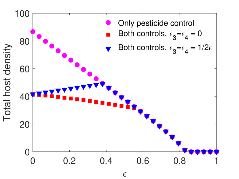
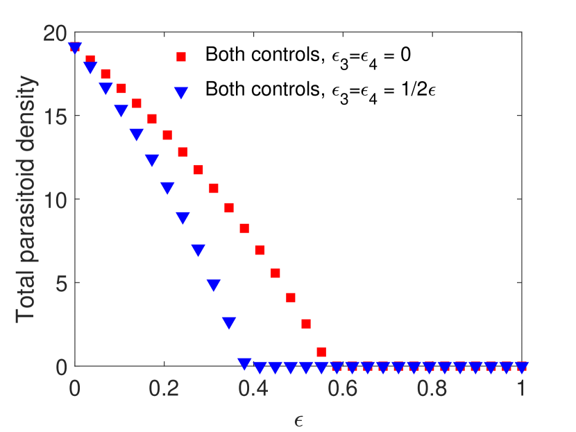
(A comparison of combined control strategies). For models (11) and (12), we consider varying the pesticide-induced mortality in the host assuming equal impact on both stages (${ϵ}_1={ϵ}_2=ϵ$). We suppose that either both stages of the parasitoid are not directly impacted by the pesticides (${ϵ}_3={ϵ}_4=0$) or the two stages are impacted but not as significantly as the host (${ϵ}_3={ϵ}_4=\frac{ϵ}{2}).$ All other parameters are fixed at the following values:

$f_0=400,s_1=0.1,s_2=0.1,s_3=0.1,s_4=0.1,c=5,$

${\beta }_1=0.9,{\beta }_2=0.9,{\gamma }_1=0.9,{\gamma }_3=0.3,a_1=1,a_2=1.$

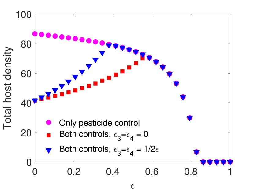
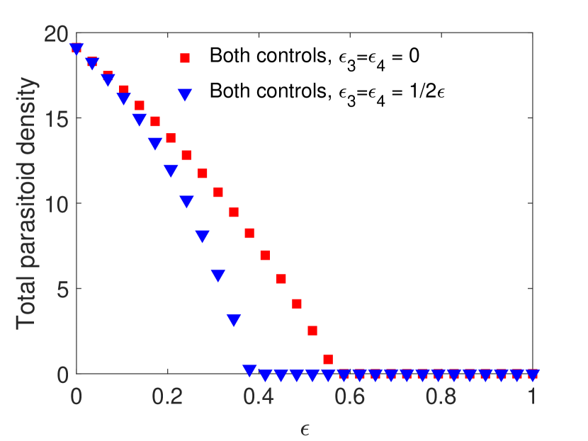
For this choice of parameters, solutions are attracted to stable equilibria for all values of $ϵ$. Notice that in Figure 1(a) and 1(c), parasitoids alone can never eradicate the host without supplementing additional parasitoids. We find that when the spraying occurs at the end of the time unit, if the pesticides do not directly impact the parasitoids, then host density decreases with the increase of pesticide concentration. However, when the pesticide directly affects the parasitoids, we notice a moderate increase in the host density for lower pesticide concentrations, but it does not exceed the host density with only chemical control (Figure 1(a)). Conversely, when spraying occurs at the beginning of the time unit, combining the two control measures produces worse results than a single biological control for lower pesticide concentration, host goes extinct for larger pesticide concentrations. This occurs even when the chemical control has no direct effects on the parasitoid due to increased indirect mortality (Figure 1(c)).

(a)

(b)

(c)

(d)

Figure 1. Shown are the bifurcation diagrams for pesticide spraying at the end of the time unit (a)-(b) and pesticide spraying at the beginning of the time unit (c)-(d). These diagrams are obtained by finding the time series solution out to time 20,000 for initial conditions $H_1(0)=H_2(0)=P_1(0)=P_2(0)=1$ using parameter values provided in Example 4.1. We consider three cases: only chemical control is applied($P_1(t)=P_2(t)=0$) (magenta circle), both chemical and biological controls are applied with no direct pesticide effect on the parasitoids(${ϵ}_3={ϵ}_4=0$) (red square), both chemical and biological controls are applied with a direct effect on the parasitoids (${ϵ}_3={ϵ}_4=ϵ/2$) (blue triangle).

However, this pattern can change when parameters are chosen such that the model exhibits oscillatory behavior. This is shown in Figure 2 with all the parameters kept the same as in Figure 1 except the host fecundity $f_0$ has been increased to 4000. This increase in $f_0$ results in stable oscillatory dynamics for smaller values of $ϵ$. In particular, for both models when ${ϵ}_3={ϵ}_4=0$, we observe oscillations for , and for both models when ${ϵ}_3={ϵ}_4=\frac{ϵ}{2}$, oscillations occur when . Interestingly, we observe a larger parasitoid density in the oscillatory region when parasitoids experience greater mortality. This increase in parasitoid density results in a subsequent decrease in the host density for both cases. But when parasitoids start decreasing, we notice an increasing trend in the host density, and the host goes extinct for sufficiently strong pesticide spray.

(a)

(b)

(c)

(d)

Figure 2. Shown are the bifurcation diagrams for pesticide spraying at the end of the time unit (a)-(b) and pesticide spraying at the beginning of the time unit (c)-(d). These diagrams are obtained by finding the time series solution out to time 20,000 for initial conditions $H_1(0)=H_2(0)=P_1(0)=P_2(0)=1$ using parameter values provided in Example 4.1 except the host fecundity is increased to $f_0=4000$. We then plot the average host and parasitoid densities using the last 500 time units. We consider three cases: only chemical control is applied ($P_1(t)=P_2(t)=0$) (magenta circle), both chemical and biological controls are applied with no direct pesticide effect on the parasitoids (${ϵ}_3={ϵ}_4=0$) (red square), both chemical and biological controls are applied with a direct effect on the parasitoids (${ϵ}_3={ϵ}_4=ϵ/2$) (blue triangle).

Example 4.2.

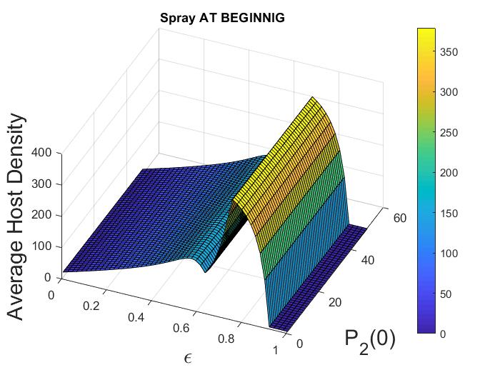
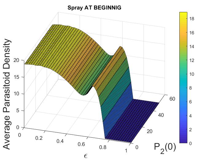
(Impact of varying control strategies on both species). In this example, we consider the impact of varying combined control parameters, i.e., pesticide spraying $ϵ$ and initial adult parasitoid density $P_2(0)$, when the pesticide equally impacts both host and parasitoid populations (i.e., ${ϵ}_1={ϵ}_2={ϵ}_3={ϵ}_4=ϵ$). We fix the parameters at the following values:

$f_0=3500,s_1=0.31,s_2=0.41,s_3=0.94,s_4=0.93,c=9,$

${\beta }_1=1.3,{\beta }_2=1.8,{\gamma }_1=0.13,{\gamma }_3=0.95,a_1=0.1,a_2=0.5.$

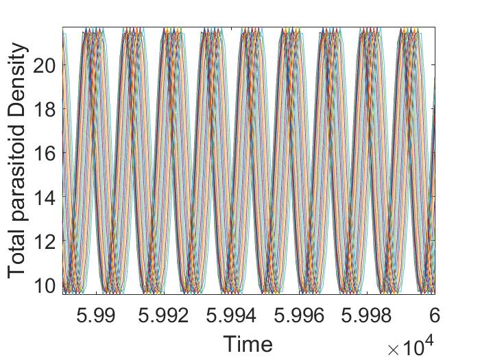
For this parameter choice, model (12) exhibits oscillatory dynamics. Here we consider the case when pesticide spraying occurs at the beginning of the time unit only. If we fix any $ϵ$, we observe that average host and parasitoid density does not vary with the initial adult parasitoid density $P_2(0)$ (Figure 3(a), 3(b)). However, if we fix any $P_2(0)$, with increasing pesticide spraying $ϵ$, we notice an increasing pattern in host density (Figure 3(a)) but a decreasing pattern in parasitoid density (Figure 3(b)) when $ϵ\le 0.6$. This trend does not follow after that. We also find that there are regions where varying $P_2(0)$ results in multiple attractors. Specifically, if we fix a $ϵ=0.63$, and keep all the parameters fixed as before, we find there are multiple attractors with similar amplitudes for $P_2(0)=1:1:20$ (Figure 3(c), 3(d)). These multiple stable attractors, all similar in amplitude, keep the Figures 3(a), 3(b) smooth in all regions. This existence of multiple attractors indicates the system dynamics are quite complicated in the intermediate $ϵ$ region, but the system has only an equilibrium attractor in the higher $ϵ$ parameter space. Similar scenarios are observed when spraying occurs at the end of the time unit (not shown).

(a)

(b)

(c)

(d)

Figure 3. (a)-(b) The average host and parasitoid density against $ϵ$ and $P_2(0)$ obtained from the last 100,000 values of 600,000 time unit simulation, when pesticide spraying occurs at the beginning of the time unit. These graphs use $H_1(0)=H_2(0)=P_1(0)=1$, with all other parameters given in Example 4.2. (c)-(d) The time series solution when $ϵ=0.6327$ for initial parasitoid density $P_2(0)=1:1:20.$)

5. Concluding Remarks

Modeling with stage structure is particularly useful because it enables us to examine how different life stages of species interact and how these interactions might be affected by external factors such as pesticides. Assuming only adult parasitoids are capable of parasitizing the hosts, we developed a discrete-time host-parasitoid model with stage structure in both species, which allows us to account for various factors, including developmental processes, differential susceptibility to pesticides, and the impact of these factors on the interactions between the host and parasitoid species.

After establishing the equilibria dynamics and persistence of the system, we explored different continuous integrated pest management (IPM) scenarios, which provide valuable insights into how the system’s dynamics are affected by different pest control strategies. First, we assumed continuous application of pesticides that occurs each time unit, such as daily spraying. Continuous pesticide spraying can significantly impact both the target pest and the parasitoid species, and the model would help us to understand the long-term consequences of such a strategy, but it might not be very realistic, especially if the unit of time in the model is a day.

We observe that the effectiveness of integrated pest management strategies depends on several factors, including the timing of the pesticide spray, pesticide susceptibility of the parasitoids, and the solutions of the system converging. In particular, when the pesticide spraying occurs continuously, spraying at the beginning of the time unit produces larger host densities than spraying at the end of the time unit and if pesticides affect parasitoids directly, pest density increases if the pesticide is not sufficiently effective (i.e. if ${ϵ}_i$ is not high enough).

Interestingly, we notice that if parasitoids are moderately affected by pesticides, then parasitoids density increases with the increase of pesticide-induced mortality. However, this higher density of parasitoids does not necessarily translate into lower host density (Figure 2). We observed that with continuous control it is possible for the combination of chemical control and natural enemies to produce worse outcomes in terms of host control than natural enemies alone if the chemical control is not sufficiently effective. In particular, when the pesticide affects natural enemies directly, a combination of biological and chemical control produces larger host densities than biological control alone when pesticides are not sufficiently effective. Of course, additional factors may further complicate the outcomes, such as the development of resistance to the pesticide ([liang2018discrete]) or coevolution between host parasitoid ([sasaki1999model]).