Chapter 4 Host-Parasitoid Model with Periodic Impulsive Effects

1. Introduction

In this chapter, we extend the host parasitoid system (LABEL:HP_equation) to an impulsive system. This formulation allows us to incorporate periodic control measures such as periodic pesticide spraying and additional parasitoid releases and its impact in the system. Using this approach, we examine how periodic interventions influence the dynamics of the system, particularly when the population exhibits oscillatory behavior. In Chapter LABEL:chapter2, we observe, it is possible that combination of continuous control measures produce worse outcome than single biological control alone when pesticide control is not sufficiently effective. However, more realistically we may expect chemical controls to be applied periodically rather than continuously. Additionally, we expect the susceptibility of the parasitoids to pesticides may be an essential factor in reducing the host population density.

In Section 3, we establish the conditions under which host eradication is achieved using these two control measures as well as conditions under which host eradication is unsuccessful resulting in the persistence of both species. Finally, in Section 4, we provide numerical examples to show how the combination of biological and chemical controls affects the pest population.

2. The Impulsive Host-Parasitoid Model

We extend model (LABEL:HP_equation) to an impulsive difference equation that includes periodic pesticide spraying along with additional periodic releases of parasitoids. This extension is obtained by following a model formulation similar to that studied in [39]. We assume at every $q$th time step there is a perturbation which incorporates a proportional decrease of the host and parasitoid populations due to applying pesticide and a constant increase in parasitoid density due to constant parasitoid release which is independent of the current parasitoid density. This perturbation is assumed to occur at the end of the time unit. The model is given by the following system of difference equations:

(1)

where, $q$ is a fixed integer and denotes the period of the impulsive effect, which means that an integrated control strategy should be applied when $t=qk$ for $k=1,2,\mathrm{\dots }$. Here ${ϵ}_i$ for $i=1,2,3,4$ denotes the proportional mortality after spraying the pesticide, and ${\tau }_i\ge 0$ for $i=1,2$ is the number of juvenile and adult parasitoids released. $H_{i,qk}$ and $P_{j,qk}$ are the densities of the host and parasitoid at time $qk$ before the impulsive perturbation, and $H_{i,q{k}^{+}}$ and $P_{j,q{k}^{+}}$ are the densities of host and parasitoid at time $qk$ after an impulsive perturbation for $i=1,2$ and $j=3,4$. The initial conditions are $(H_1(0^{+}),H_2(0^{+}),P_1(0^{+}),P_2(0^{+})=(H_1(0),H_1(0),P_1(0),P_2(0)$. Here for convenience, we denote the initial density after an impulsive perturbation at time $t=0$. Note that if $q=1$ and ${\tau }_1={\tau }_2=0$, then the system (1) is equivalent to the continuous model with spraying at the end of the time interval, as given by system (LABEL:toxicant_at_end).

In Lemma 1, we first verify that solutions of system (1) are point-dissipative.

Lemma 1.

There exists a compact set $B_p$ that attracts all solutions of (1).

Proof.

Consider, $t$ in the impulsive interval, i.e., $t\in [q{s}^{+},q(s+1))$. Then by the assumption on $f$ we can write,

$$H_{1,q{(s+1)}^{+}}\le \frac{D(1-{ϵ}_1)(1-{(s_1(1-{\gamma }_1))}^q)}{1-s_1(1-{\gamma }_1)}+(1-{ϵ}_1){(s_1(1-{\gamma }_1))}^q{H}_{1,q{s}^{+}}.$$

It follows that

$$\underset{s\to \mathrm{\infty }}{lim\; sup}{H}_{1,q{s}^{+}}\le \frac{D(1-{ϵ}_1)(1-{(s_1(1-{\gamma }_1))}^q}{(1-s_1(1-{\gamma }_1))(1-(1-{ϵ}_1){(s_1(1-{\gamma }_1))}^q)}:=\widetilde{H_1}.$$

Thus for any $\eta >0$, there exists a $T_1>0,$ which depends on $H_1^{+}(0)$, such that for $s>T_1$,

$$H_{1,qs+}\le \widetilde{H_1}(1+\eta ).$$

Similarly, from the second equation of system (1) we have,

$$H_{2,q{(s+1)}^{+}}\le \frac{s_1{\gamma }_1\widetilde{H_1}(1+\eta )(1-{ϵ}_2)(1-s_2^q)}{1-s_2}+s_2^q(1-{ϵ}_2)H_{2,q{s}^{+}},$$

which implies after taking ${\eta }^{+}\to 0$,

$$\underset{s\to \mathrm{\infty }}{lim\; sup}{H}_{1,q{s}^{+}}\le \frac{s_1{\gamma }_1\widetilde{H_1}(1-{ϵ}_2)(1-s_2^q)}{(1-s_2)(1-s_2^q(1-{ϵ}_2))}:=\widetilde{H_2}.$$

Thus for any $\eta >0$, there exists a $T_2>0,$ which depends on $H_2^{+}(0)$, such that for $s>T_2$,

$$H_{2,q{s}^{+}}\le \widetilde{H_2}(1+\eta ).$$

Then for any $s>T_2,$

$$P_{1,q{(s+1)}^{+}}\le \frac{(1-{ϵ}_3)({\beta }_1\widetilde{H_1}+{\beta }_2\widetilde{H_2})(1+\eta ){(1-s_3(1-{\gamma }_3))}^q}{(1-s_3(1-{\gamma }_3))}+(1-{ϵ}_3){(s_3(1-{\gamma }_3))}^q{P}_{1,q{s}^{+}}+{\tau }_1,$$

which implies

$$\underset{s\to \mathrm{\infty }}{lim\; sup}{P}_{1,q{s}^{+}}\le \frac{(1-{ϵ}_3)({\beta }_1\widetilde{H_1}+{\beta }_2\widetilde{H_2}){(1-s_3(1-{\gamma }_3))}^q+{\tau }_1(1-s_3(1-{\gamma }_3))}{(1-s_3(1-{\gamma }_3))(1-(1-{ϵ}_3){(s_3(1-{\gamma }_3))}^q)}:=\widetilde{P_1},$$

after taking ${\eta }^{+}\to 0.$ Thus there exists a $T_3\ge T_2$, which depends on $P_1^{+}(0),$ such that for $s>T_3,$

$$P_{2,q{(s+1)}^{+}}\le \frac{s_3{\gamma }_3(1-{ϵ}_4)(\widetilde{P_1}+\eta )(1-s_4^q)}{(1-s_4)}+s_4^q(1-{ϵ}_4)P_{1,q{s}^{+}}+{\tau }_2,$$

It follows from an analogous argument that,

$$\underset{s\to \mathrm{\infty }}{lim\; sup}{P}_{2,q{s}^{+}}\le \frac{s_3{\gamma }_3(1-{ϵ}_4)\widetilde{P_1}(1-s_4^q)+{\tau }_2(1-s_4)}{(1-s_4)(1-s_4^q(1-{ϵ}_4)}:=\widetilde{P_2}.$$

We define a compact set $B_p:=\{(H_1,H_2,P_1,P_2)\in {ℝ}_{+}^4:0\le H_1\le \widetilde{H_1},0\le H_2\le \widetilde{H_2},0\le P_1\le \widetilde{P_1},0\le P_2\le \widetilde{P_2}\}$. Then $B_p$ attracts all solutions of the system (1). Hence, the system (1) is point-dissipative. ∎

3. Existence and Global Stability of Host-Eradication Periodic Solutions

Next, we determine when system (1) results in host eradication. For this, we consider the existence and stability of a host-eradication periodic solution of system (1). We first consider the parasitoid-only system:

(2)

In Lemma 2, we show that all solutions of system (2) converge to a unique non-trivial periodic solution.

Lemma 2.

System (2) has a periodic solution $P_t^{\ast }$ and, for every solution $P_t$ of (2), we have $|P_t-P_t^{\ast }|\to 0$ as $t\to \mathrm{\infty }$, where $P_t^{\ast }$ is defined as

(3)

$t\in [q{s}^{+},q(s+1)),s=0,1,2\mathrm{\dots },$ and

$$\left(\begin{array}{c}{P}_1(0)\\ P_2(0)\end{array}\right):=\left(\begin{array}{c}\frac{{\tau }_1}{1-s_3^q(1-{ϵ}_3){(1-{\gamma }_3)}^q}\\ \frac{s_3{\gamma }_3{\tau }_1(1-{ϵ}_4){\sum }_{n=0}^{q-1}{s}_4^n{(s_3(1-{\gamma }_3))}^{q-1-n}}{(1-s_3^q{(1-{\gamma }_3)}^q(1-{ϵ}_3))(1-s_4^q(1-{ϵ}_4))}+\frac{{\tau }_2}{(1-s_4^q(1-{ϵ}_4))}\end{array}\right).$$

In particular, if ${\tau }_1>0$, then this periodic solution is always positive.

Proof.

It follows from the periodicity of the system (2) that the solution can be defined at the impulsive sub-interval $t\in [q{s}^{+},q(s+1))$ with $s=0,1,2\mathrm{\dots }$, and $t=q{s}^{+}$ means that we take the density of the parasitoids after an impulsive perturbation as the initial value in this interval.
For any $t\in [q{s}^{+},q(s+1))$, it follows from system (2) that

If $t=q(s+1)-1$, then we have,

Applying the impulsive condition that we have

or equivalently,

(4)

Therefore, the existence of periodic solution of the system (2) with period $q$ implies that the difference equation (2) has a steady state satisfying,

Solving the system we find,

$$P_{1,0}=\frac{{\tau }_1}{1-s_3^q(1-{ϵ}_3){(1-{\gamma }_3)}^q},$$

and

$$P_{2,0}=\frac{s_3{\gamma }_3{\tau }_1(1-{ϵ}_4){\sum }_{n=0}^{q-1}{s}_4^n{(s_3(1-{\gamma }_3))}^{q-1-n}}{(1-s_3^q{(1-{\gamma }_3)}^q(1-{ϵ}_3))(1-s_4^q(1-{ϵ}_4))}+\frac{{\tau }_2}{(1-s_4^q(1-{ϵ}_4))}.$$

Hence, there exists a periodic solution of the system (2). Note that restrictions on the model parameters mean these two quantities always positive for ${\tau }_1>0$.

Next, we note that the convergence of solutions to the periodic solution $P_t^{\ast }$ follows from the linearity of the projection matrix in equation (4) and the fact that the eigenvalues of this matrix have absolute value less than 1. Specifically, define,

By iterating Equation (4), we obtain

$P(q{(s+1)}^{+})=A_p^{s+1}P(0)+{\displaystyle \sum _{i=0}^s}{A}_p^{s-i}\tau .$

Since , taking the limit as $s\to \mathrm{\infty }$ we find that the solution converges to ${(I-A_p)}^{-1}\tau$ which is the equilibrium solution to equation (4). ∎

Next, we establish the global attractivity of the host eradication cycle.

Theorem 1.

The host eradication cycle $(0,0,P_{1,t}^{\ast },P_{2,t}^{\ast })$ of model (1) is globally attracting if

(5)

In particular, a sufficient condition is

(6)

where $\tilde{a}:=\text{min}\{a_1,a_2\}$ and $\widetilde{ϵ}:=\text{min}\{{ϵ}_1,{ϵ}_2\}$.

Proof.

Note that,

Consider the following impulsive difference equation,

(7)

where, $t=0,1,2,\mathrm{\dots }$ and $k=1,2,\mathrm{\dots }$ It follows from Lemma 2 that if we have $P_1(0)=Q_1(0)$ and $P_2(0)=Q_2(0)$, then we have $P_1(t)\ge Q_1(t)$ and $P_2(t)\ge Q_2(t)$, and $Q_1(t)\to P_1^{\ast }(t)$ and $Q_2(t)\to P_2^{\ast }(t)$ as $t\to \mathrm{\infty }.$ Hence, for any $\delta >0$ there exists a $t_0>0$ such that $P_1(t)\ge Q_1(t)>P_1^{\ast }(t)-\delta$, $P_2(t)\ge Q_2(t)>P_2^{\ast }(t)-\delta$, holds true for large $t\ge t_0$. Therefore, for $t\ge t_0$ we have

(8)

After the impulse it follows that,

Taking $\tilde{a}:=\text{min}\{a_1,a_2\},\widetilde{ϵ}:=\text{min}\{{ϵ}_1,{ϵ}_2\}$ we have a sufficient condition,

(9) ${\left(\begin{array}{c}{H}_1\\ H_2\end{array}\right)}_{q{(s+1)}^{+}}\le {\lambda }^q(1-\widetilde{ϵ}){\displaystyle \prod _{t=qs}^{q(s+1)-1}}{e}^{-\tilde{a}(P_2^{\ast }(t)-\delta )}{\left(\begin{array}{c}{H}_1\\ H_2\end{array}\right)}_{q{s}^{+}},$

where $\lambda =\rho [A_h(0,0,0,0)]$. Assume, inequality (5), (6) holds true. Then there exists a $\delta >0$ sufficiently small such that

and

Then $H_{1,q{s}^{+}}\to 0$, $H_{2,q{s}^{+}}\to 0$ as $s\to \mathrm{\infty }.$
It follows from model (1) that

For any $t\in [q{s}^{+},q(s+1))$, we have,

Therefore, $H_1\to 0$ and $H_2\to 0$ as $t\to \mathrm{\infty }.$ This completes the proof. ∎

Next, we provide conditions for the persistence of the host and parasitoid for system (1). Let, $E_p^0=(0,0,P_1^0,P_2^0)$, $E_p^1=(0,0,P_1^1,P_2^1)$… $E_p^{q-1}=(0,0,P_1^{q-1},P_2^{q-1})$ be the host-free $q$ -periodic solution, which we can obtain from the equation (3) defined in Lemma 2 and define the matrix continuous in $z=(x,y)$ and $\xi$ to be

where, $x:=(H_1,H_2)$, $y:=(P_1,P_2)$, and $\xi$ is the bounded set of parameter vectors for system (1). Let ${\mathrm{\Re }}_p$ be the spectral radius of the product of matrices $A_h(q+qs-1,E_p^{q-1})A_h(q+qs-2,E_p^1)\mathrm{\dots }{A}_h(q{s}^{+},E_p^0)$. Specifically,

(10) $${\mathrm{\Re }}_p=\rho [A_h(q+qs-1,E_p^{q-1})A_h(q+qs-2,E_p^1)\mathrm{\dots }{A}_h(q{s}^{+},E_p^0)],$$

which is equivalent to equation (5). The solutions corresponding to a fixed parameter set ${\xi }_0$ are denoted by $(H_1(t),)H_2(t),P_1(t),P_2(t))$ while solutions corresponding to any other parameter set $\xi$ are denoted by $(H_1^{\xi }(t),)H_2^{\xi }(t),P_1^{\xi }(t),P_2^{\xi }(t)).$

Theorem 2.

If ${\mathrm{\Re }}_p>1$ then there exists ${ϵ}_{hp}>0$ and a bounded neighborhood $N_{\xi 0}$ of ${\xi }_0$ such that

(11) $$\underset{t\to \mathrm{\infty }}{lim\; inf}\text{min}(H_1^{\xi }(t),H_2^{\xi }(t),P_1^{\xi }(t),P_2^{\xi }(t))>{ϵ}_{hp},$$

for all solutions $(H_1^{\xi }(t),H_2^{\xi }(t),P_1^{\xi }(t),P_2^{\xi }(t))$ of system (1), with $t\ge s_0$, where $s_0$ is the initial time and $\xi \in N_{\xi 0}$ with $H_1^{\xi }(0)+H_2^{\xi }(0)>0$ and ${\tau }_1>0$.

Proof.

First, to prove the robust uniform host-persistence for the system (1) we write the model (1) as,

(12)

where $F(t,z,\xi )=(A_h(t,z,\xi )x,f(t,z,\xi ))$ denotes the right hand side of the system and $\xi \in {ℝ}^l$, where $l\in ℝ$ denotes the parameter vector. We define,

and

for $k=1,2,\mathrm{\dots }$, where $i=1,2,3,4$ and $j=1,2$. Define the following system which is linear in $u$

(13) $$u(t+1)=A_h(t,z(t),\xi )u(t),$$

where $z(t)$ is the solution of (12), $z(s_0)=z_0$, and $P(t+s_0,s_0,z_0,\xi )$ is the solution matrix for the linear system (13) in $u$, where $u\in {ℝ}_{+}^2$ and $P(s_0,s_0,z_0)=I$. Define the state space $Z=:\{(x,y)\in {ℝ}_{+}^4|x\ge 0,y\ge 0\}$, the extinction set $X:=\{(x,y)\in {ℝ}_{+}^4:x(t)=0\forall t>0\}$ and let $B_p$ is a compact set defined in Theorem 1. Let, $M=B_p\cap X$. Now we verify the assumptions (D) and (H1)-(H5) from [salceanu2013robust] for the model (12) when $t\in [q{s}^{+},q(s+1))$ for $s=0,1,2\mathrm{\dots }$. For the reader’s convenience, the assumptions are given in the Appendix B. Now to verify assumption (D), fix ${\xi }_0\in N_{{\xi }_0}$, $t_0\in {\mathbb{Z}}_{+}$, and $\eta \in U$. Then utilizing the primitivity of the matrix $A_h(x,y,\xi )$ and for finitely many $s_0\in [q{s}^{+},q(s+1))$, we can choose a $C$ such that $|P(t_0+s_0,s_0,z_0,{\xi }_0)\eta |\ge C$ holds. Hence, Assumption (D) holds.

Next, Assumptions (H1) and (H5) hold from the dissipativity of the system (1), which follows from Theorem 1. Since the dynamics on $X$ are given by model (2), by Lemma 2, for every $z_0\in M$ and $\forall s_0\in {\mathbb{Z}}_{+}$, $P_1(t)\to P_1^{\ast }(t)$ and $P_2(t)\to P_2^{\ast }(t)$ as $t\to \mathrm{\infty }$, which are independent of initial time $s_0$. Since this holds for all $t\in {\mathbb{Z}}_{+},$ then it holds for any $t\in [0,t_0]$. Hence (H3) holds. To satisfy Assumption (H4), it is trivial to find a $K$ such that $\Vert A_h(t,z_0,{\xi }_0)\Vert \le K$ holds $\forall t\in {\mathbb{Z}}_{+}$, $\forall z_0\in \tilde{M}\subset X$ and $\forall {\xi }_0\in \widetilde{N_{{\xi }_0}}$, where $\tilde{M}$ is any compact set in $X$. Now, every entry of $A_h(t,z(t),{\xi }_0)$ and $F=(A_h(t,z(t),{\xi }_0)x,f)$ from the map (12) are $C^1$ in $z$ and $\xi$ where $z\in \tilde{M}\subset X$ and $\xi \in \widetilde{N_{{\xi }_0}}$. Thus, equations (LABEL:F)-(LABEL:A1) from Assumption (H4) are satisfied, and also equation (LABEL:phi) holds from dissipativity of system (1). Hence assumption (H4) holds. Now, it remains to verify the Assumption (H2). Note, by Lemma 2, $\forall z_0\in M$, all orbits of system (2) are attracted to the $q$-periodic orbit $𝒫=\{E_p^0,E_p^1,E_p^2,\mathrm{\dots },E_p^{q-1}\}$ for any $s_0>0$. For simplicity, we write $A(t,z,{\xi }_0)$ as $A(t,z)$ and $P(t,s_0,z_0,{\xi }_0)$ as $P(t,s_0,z_0)$. Next, we calculate the spectral radius of the solution matrices for each periodic orbit of system (2) in the impulsive interval,

$P(q+qs,q{s}^{+},E_p^0)=$ $A_h(q+qs-1,E{p}^{q-1})\mathrm{\dots }{A}_h(qs+1,E{p}^1)A_h(qs+,E_p^0),$

$P(q+qs+1,qs+1,E_p^1)=$ $A_h(q+qs,E_p^0)\mathrm{\dots }{A}_h(qs+2,E_p^2)A_h(qs+1,E_p^1),$

$P(q+qs+2,qs+2,E_p^2)=$ $A_h(q+qs+1,E_p^1)\mathrm{\dots }{A}_h(qs+3,E_p^3)A_h(qs+2,E_p^2),$

$\mathrm{⋮}$

$P(2q+qs-1,qs+q-1,E_p^{q-1})=$ $A_h(2q+qs-2,E_p^{q-2})\mathrm{\dots }{A}_h(qs+q,E_p^0)A_h(qs+q-1,E_p^{q-1}).$

All the solution matrices are primitive and have same spectral radius ${\mathrm{\Re }}_p$ by the Lemma 4.5 in [salceanu2011robust], which is greater than one by hypothesis. Then by the Perron-Frobenius theorem, all solution matrices have positive left eigenvectors corresponding to the spectral radius ${\mathrm{\Re }}_p>1$. Then Proposition 3.8 in [salceanu2013robust] says that (A2) holds. Thus, from Theorem 3.5 in [salceanu2013robust] we obtain that the total host population for the system (1) is robustly uniformly persistent, i.e. there exists an ${ϵ}_h>0$ and a bounded neighbourhood $N_{\xi 0}$ of ${\xi }_0$ such that

$$\underset{t\to \mathrm{\infty }}{lim\; inf}(|H_1^{\xi }(t)|+|H_2^{\xi }(t)|)>{ϵ}_h,$$

satisfying $\xi \in N_{\xi 0}$, $H_1^{\xi }(0)+H_2^{\xi }(0)>0$. Then, using the equations for $H_1\text{and}{H}_2$ in system (1), we obtain,

$$\underset{t\to \mathrm{\infty }}{lim\; inf}|H_1^{\xi }(t)|>{ϵ}_{h1}>0,\text{and}\underset{t\to \mathrm{\infty }}{lim\; inf}|H_2^{\xi }(t)|>{ϵ}_{h2}>0,$$

which implies,

(14) $$\underset{t\to \mathrm{\infty }}{lim\; inf}\text{min}(H_1^{\xi }(t)+H_2^{\xi }(t))>{\widetilde{ϵ}}_h>0,$$

for all solutions $(H_1^{\xi }(t),H_2^{\xi }(t),P_1^{\xi }(t),P_2^{\xi }(t))$ of system (1), with $t\ge s_0$ and $\xi \in N_{\xi 0}$ with $H_1^{\xi }(0)+H_2^{\xi }(0)>0.$ To prove the parasitoid persistence for system (1), by Lemma 2 that if we have $P_1(0)=Q_1(0)$ and $P_2(0)=Q_2(0)$, then we have $P_1(t)\ge Q_1(t)$ and $P_2(t)\ge Q_2(t)$ and $Q_1(t)\to P_1^{\ast }(t)$ and $Q_2(t)\to P_2^{\ast }(t)$ as $t\to \mathrm{\infty }$, which are positive if ${\tau }_1>0$, where $P(t)$ is the solution of (1) and $Q(t)$ is the solution of the system (2). Then, there exists a ${ϵ}_{p1}>0,{ϵ}_{p2}>0$ and $N_{{\xi }_0}$, a bounded neighbourhood of ${\xi }_0$ such that

$$\underset{t\to \mathrm{\infty }}{lim\; inf}{P}_1^{\xi }(t)>{ϵ}_{p1},\text{and}\underset{t\to \mathrm{\infty }}{lim\; inf}{P}_2^{\xi }(t)>{ϵ}_{p2},$$

satisfying $\xi \in N_{\xi 0}$, which implies,

(15) $$\underset{t\to \mathrm{\infty }}{lim\; inf}\text{min}(P_1^{\xi }(t)+P_2^{\xi }(t))>{\widetilde{ϵ}}_p>0,$$

for all solutions $(H_1^{\xi }(t),H_2^{\xi }(t),P_1^{\xi }(t),P_2^{\xi }(t))$ of system (1), with $t\ge s_0$ and $\xi \in N_{\xi 0}$ with ${\tau }_1>0.$ Then equation (11) follows from equations (14) and (15) letting ${ϵ}_{hp}:=\text{min}\{\widetilde{{ϵ}_h},\widetilde{{ϵ}_p}\}.$ ∎

4. Numerical Study of the Impulsive Model

In this section, we consider some numerical examples of the impulsive model (1). In Example 4.1, we compare the impact of combined control strategies when the control measures are applied periodically at the same time units. Next, in Example 4.2, we compare this to the application of combined control measures in different time units. Then, in Example 4.3, we consider how different control measures result in different average host densities. We find that for some parameter ranges for which multiple attractors occur, host control effectiveness is initial condition dependent.

Example 4.1.

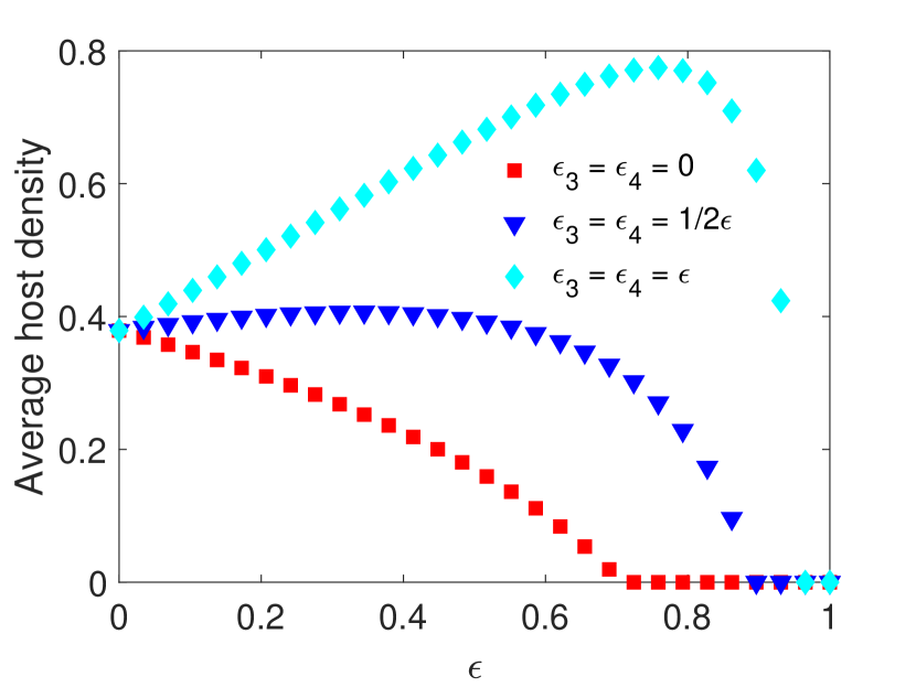
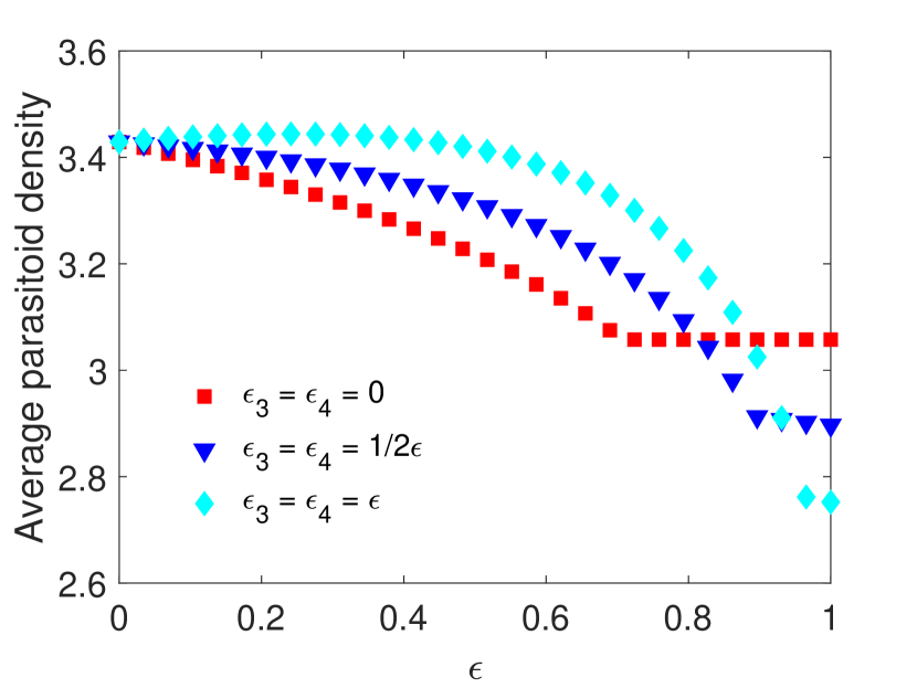
(Impact of combined periodic control strategies). For the impulsive model (1), we consider the impact of varying pesticide-induced mortality in the host, assuming equal impacts on both stages, i.e., ${ϵ}_1={ϵ}_2=ϵ$. We consider three scenarios: pesticide spraying does not directly impact the parasitoid (${ϵ}_3={ϵ}_4=0$), has moderate impacts on the parasitoid (${ϵ}_3={ϵ}_4=\frac{ϵ}{2}$) and has severe impacts on the parasitoids (${ϵ}_3={ϵ}_4=ϵ$). All other parameters are fixed at the following values:

$f_0=500,s_1=0.71,s_2=0.71,s_3=0.71,s_4=0.72,c=5,$

${\beta }_1=0.3,{\beta }_2=0.3,{\gamma }_1=0.93,{\gamma }_3=0.25,a_1=1,a_2=1,$

$q=7,{\tau }_1=1,{\tau }_2=5.$

We observe that when pesticides do not impact the parasitoids directly, the average host density decreases with increasing pesticide concentration (Figure 1(a)). Since the impulsive model corresponds to spraying at the end of the time unit, this agrees with the dynamics observed in Example LABEL:equilibrium_example (Figure LABEL:equilibrium_example_figure_A). Meanwhile, when pesticides result in moderate direct mortality in parasitoids, we observe that the average host density stays roughly the same for weak pesticide effects, while the host goes extinct for sufficiently intense pesticide effects. However, when the direct impact of pesticides on parasitoids is severe, the average host density increases with increasing pesticide concentration, resulting in host density almost doubling in certain situations. We also noticed that due to parasitoid supplementation, the parasitoid population survives after the hosts die out (Figure 1(b)). Interestingly, parasitoid density becomes larger when they experience greater mortality (Figure 1(b)). However, this larger parasitoid density does not result in a lower average host density.

(a)

(b)

Figure 1. Shown are the bifurcation diagrams for the impulsive system (1) when control meansures are applied in the same time units. These diagrams are obtained by finding the time series solution out to time 5,000 for initial conditions $H_1(0)=H_2(0)=P_1(0)=P_2(0)=1$ using the parameter values provided in Example 4.1. We then plot the average host and parasitoid densities using the last 500 time units. We consider three cases: no direct pesticide effect on parasitoid ( ${ϵ}_3={ϵ}_4=0$) (red square), moderate direct pesticide impact on parasitoids (${ϵ}_3={ϵ}_4=\frac{ϵ}{2}$) (blue triangle), severe direct pesticide impact on parasitoids (${ϵ}_3={ϵ}_4=ϵ$) (cyan diamond).

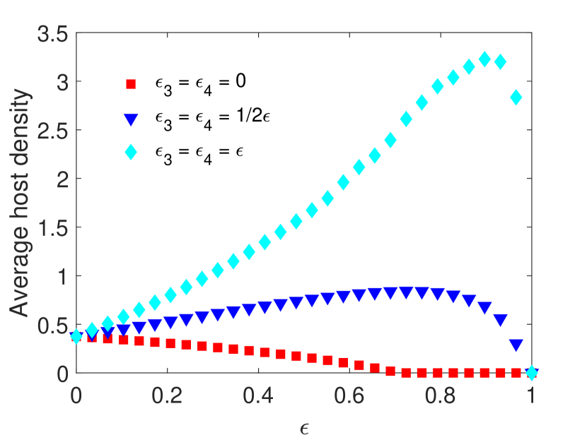
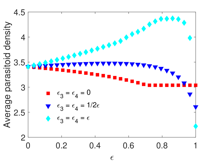
Example 4.2.

(Impact of combined periodic control applied at different times). In this example, we consider the impact of varying pesticide-induced mortality when the combined control measures (pesticide spraying $ϵ$ and parasitoid supplementation $\tau$) are applied in different time units. We assume pesticide spraying occurs at every $q$ time unit, whereas the time between control measures applied is $r$, which means that parasitoid supplementation occurs at $q-r$ time units. All other parameters are fixed as in the Example 4.1. We compare the same three scenarios as described in Example 4.1, assuming equal pesticide impacts on both host stages $({ϵ}_1={ϵ}_2=ϵ)$. We observe that if parasitoid supplementation occurs $q-r=4$ time units after pesticide spraying, then the average host and parasitoid density increases if parasitoids experience direct mortality but have a minimal effect on host and parasitoid population density when parasitoids do not experience direct mortality (Figure 2). If we increase the time between control measures further, notice that the average host density increases more than double with the increase of the pesticide spraying, demonstrating that worse pest control outcomes occur when controls are applied at distinct time units.

(a)

(b)

Figure 2. Shown are the bifurcation diagrams for the impulsive system (1) when control measures are applied at different time units. These diagrams are obtained by finding the time series solution out to time 5,000 for initial condition $H_1(0)=H_2(0)=P_1(0)=P_2(0)=1$ using the parameter values provided in Example 4.1 and $r=3$. We then plot the average host and parasitoid densities using the last 500 time units. We consider three cases: no direct pesticide effect on parasitoid ( ${ϵ}_3={ϵ}_4=0$) (red square), moderate direct pesticide impact on parasitoids (${ϵ}_3={ϵ}_4=\frac{ϵ}{2}$) (blue triangle), and severe direct pesticide impact on parasitoids (${ϵ}_3={ϵ}_4=ϵ$) (cyan diamond).

Example 4.3.

(Impact of control strategies on host densities). In this example, we first consider the impact of varying the control parameters $q$ and ${\tau }_2$ for the impulsive model (1). All other parameters are fixed at the following values:

$f_0=140,s_1=0.11,s_2=0.11,s_3=0.54,s_4=0.83,c=0.8,$

${\beta }_1=1.3,{\beta }_2=1.8,{\gamma }_1=1.3,{\gamma }_3=0.25,a_1=0.1,a_2=0.1,$

${ϵ}_1=0.18,{ϵ}_2=0.17,{ϵ}_3=0.15,{ϵ}_4=0.15,{\tau }_1=5.$

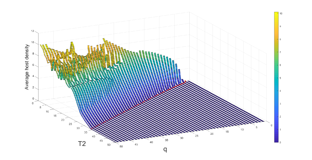
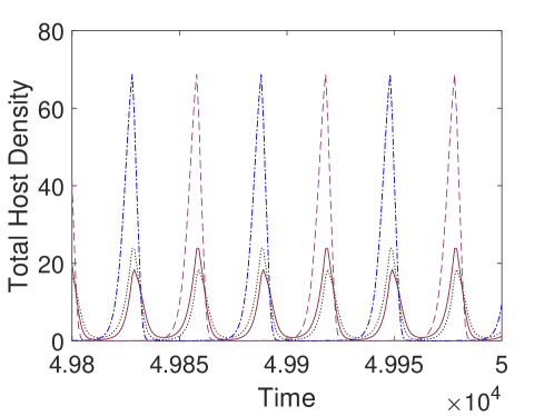
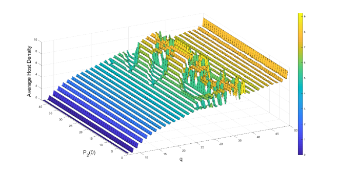
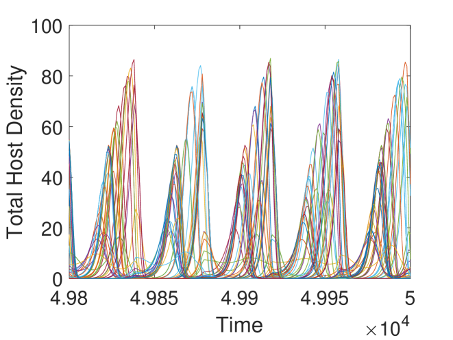
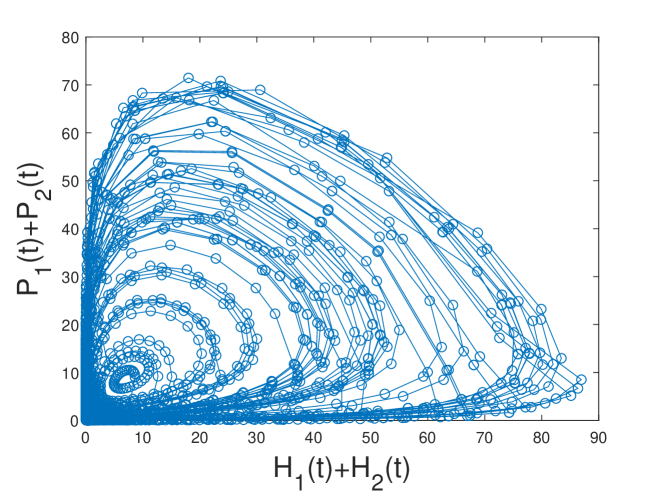
We observe in Figure 3, that the host is eradicated for sufficiently strong control measures (i.e., frequent pesticide spraying and large parasitoids release). But, when these control measures get weaker, we notice an increasing trend in the average host density. However, this increasing trend does not follow smoothly for some parameter regions. This is due to the existence of multiple attractors with significant differences in average host densities in certain regions (Figure 3(b)). To inspect this region, we fix $q=30,\text{and}{\tau }_2=4$ and keep all the parameters as before. We find four stable attractors when $0.01\le P_2(0)\le 50$ (Figure 4(b)). To examine this situation broadly, we fix ${\tau }_2=4$ and find the average host density against $q$ and $P_2(0)$ (Figure 4(a)). We observe for some parameter regions of $q$ and $P_2(0)$, the average host density changes significantly, whereas for larger $q$ values, though average host density does not change significantly, we find a large number of attractors, which implies the system dynamics are quite complicated.

(a)

(b)

Figure 3. (a) Average host density against $q$ and ${\tau }_2$ obtained from the last 100,000 values of a 500,000-time unit simulation. All parameters are given as in Example 4.3 with initial condition $H_1(0)=H_2(0)=P_1(0)=P_2(0)=1$. The red line corresponds to host eradication condition (5). Note that $q$ must be integer-valued. (b) The final time series solutions of system (1) when $q=30$ and ${\tau }_2=4$ and all other parameters are fixed as in Example 4.3. For $0.01\le P_2(0)\le 50$, the system has four stable attractors, two with large amplitudes and two with small amplitudes.

(a)

(b)

(c)

Figure 4. (a) The average host density against $P_2(0)$ and $q$ obtained from the last 100,000 values of a 500,000-time unit simulation. These graphs are obtained using ${\tau }_2=4$ and $H_1(0)=H_2(0)=P_1(0)=1$, with all other parameters are given in Example 4.3. (b) The time series solution when $q=40$ for initial adult parasitoid density $P_2(0)=1:1:50$ (c) A sample phase plane trajectory when $q=40$ and $P_2(0)=1$ consisting of the last 3000 values of a 50,000-time unit simulation.

5. Concluding Remarks

We extends the host-parasitoid model developed in Chapter LABEL:chapter2 to an impulsive difference equation system by incorporating periodic pesticide spraying. This case is more practical as it accounts for the periodic application of pesticides. We also included periodic parasitoid supplementation.

After establishing the global dynamics of the host eradication cycle and the robust persistence of the periodic host-parasitoid system, we explored the periodic integrated pest management approach. As observed in the continuous case in Chapter LABEL:chapter2, we also observed that if spraying directly affects the parasitoid species, increasing the pesticide induces mortality $ϵ$, increases the average host density, if the pesticide is not sufficiently effective. This occurs both in the case when periodic control measures are applied at the same time or at different time units. Furthermore, we observe that parasitoid density may be higher for larger direct pesticide-induced mortality (larger ${ϵ}_3$ and ${ϵ}_4$). But, this higher density does not translate the host density into a lower density (Figure 1). Additionally, we observe that the pest is eradicated with strong control measures (frequent spraying or larger amounts of parasitoid release), whereas host outbreaks or low host density persistence occur when the combination of control measures is weaker (Figure 3(a)). We also find some parameter regions where the solution of the system is initial condition dependent (Figure 4(a)). This is the result of the existence of multiple attractors (Figure 3(b)).

Finally, our results show the importance of integrated pest management (IPM) strategies and emphasizes the necessity of considering the interactions between various pest control methods. A well-planned and integrated approach to pest management is essential to achieve effective and sustainable results while minimizing pesticide effects on the natural enemies.