Chapter 5 A Discrete-Time SIS Model with Vaccination

1. Introduction

Vaccination is one of the most effective way in reducing the prevalence of infectious disease by strengthening individual immunity. When vaccination is partially effective, systems may exhibit backward bifurcation. When a system exhibits backward bifurcation at $R_0=1$, the infective population increases suddenly in number when $R_0$ increases past 1. A backward bifurcation at $R_0=1$ makes controlling the disease harder. Moreover, reducing the net reproductive number $R_0$ below one may no longer be sufficient to eradicate the disease. Instead, there is a region of $R_0$ values less than one for which the model exhibits bistability between the disease-free steady state and an endemic steady state. Therefore, it is necessary to bring $R_0$ well below one, if there is backward bifurcation at $R_0=1$.

A number of mechanisms have been shown to lead to a backward bifurcation in epidemic models. A classic example is imperfect vaccination in a continuous-time Susceptible-Infectious-Susceptible model with Vaccination (SISV) ([brauer2004backward]). For this model, it has been shown that two factors are needed for a backward bifurcation to arise when the disease-free equilibrium destabilizes: infected individuals are able to recover from the disease, returning to the susceptible class, and the vaccine does not provide full immunity from the disease. Other examples include exogenous reinfection in tuberculosis, disease-induced mortality in vector-borne diseases, vaccine-derived immunity waning, risk structured scenarios, and density-dependent disease treatment ([blayneh2010backward, garba2008backward, guerrero2018different, gumel2012causes, hadeler1997backward, wangari2018backward]).

Since disease data are typically reported at discrete time intervals, such as daily, weekly, monthly, or yearly, it is natural to consider discrete-time epidemic models for forecasting disease transmission dynamics, as they more closely reflect the structure of observed data ([yakubu2021discrete]). The goal of this chapter is to determine whether the mechanisms that causes backward bifurcation in continuous-time carry-over to the discrete-time systems.

In discre-time epidemic models, results concerning the stability of endemic equilibria are more limited, particularly for models in which infection is not incorporated as a subtracted term, as is done in continuous time (but see [castillo2001discrete, xiang2020stability]). Although such infection terms are mathematically convenient, introducing nonlinearities that are often easier to handle computationally, they can lead to negative population values in discrete-time models if additional, non-biological restrictions are not imposed. A notable advancement in this direction is [xiang2020stability], in which the local stability of an endemic equilibrium in a discrete-time SIRS model with vaccination (that provides complete immunity) for a general (non-negative) infection nonlinearity is established.

In this chapter, we develop two discrete-time formulations of a SISV model. These models differ in the assumed order of events within a discrete time unit: the first formulation assumes that vaccination occurs before disease transmission, whereas the second reverses this order. For both models, we keep the nonlinearities governing recruitment and disease infection general. However, we note that if disease transmission is described by a negative exponential term, as can be derived by assuming that infections follow a Poisson process, then it is not possible to find explicit solutions for the endemic equilibria. Therefore, we utilize a bifurcation approach to study the endemic dynamics that arise when the disease-free equilibrium destabilizes.

In keeping with the continuous-time findings, we show that the first model may exhibit a backward bifurcation provided that individuals are able to recover from the disease and the vaccine provides partial immunity. In contrast, the second model only requires the former condition and may, in fact, produce a backward bifurcation when vaccination is fully effective. Moreover, for both models we show that the disease-free equilibrium is globally asymptotically stable when disease recovery is not possible. We note that the existence of a backward bifurcation in a discrete-time SISV model was also studied in [jang2008backward]. The models presented here differ from this earlier work in that the model in [jang2008backward] assumes that all events occur simultaneously within each discrete time step. This assumption necessitates restrictions on the force of infection in order to guarantee positivity of solutions.

This chapter is organized as follows. In Section 2, we develop the first discrete-time SISV model. This model assumes that vaccination occurs before disease transmission and may only be partially effective. In Section 3, we present analysis of the SISV model. We study the local and global stability of the disease-free equilibrium and apply the bifurcation theorem from Chapter LABEL:chapter1.5 to establish conditions under which this equilibrium undergoes a backward bifurcation when the reproduction number $R_0$ increases past one. In Section 4, we compare these results to an alternative model formulation in which disease transmission occurs before vaccination. In Section 5, we present some numerical examples to illustrate the results for these two models. Finally, in Section 6, we summarize our findings and discuss future directions.

2. Model Formulation

To introduce the discrete-time SISV model, we assume at each time unit $t\in \{0,1,2,\mathrm{\dots }\},$ each member of the population is either susceptible $S,$ infectious $I$, or vaccinated $V$, where the total population size at time $t$ is given by

$$N(t)=S(t)+I(t)+V(t).$$

We define the risk of infection according to an ‘escape’ function

$$\varphi :[0,\mathrm{\infty })\to [0,1],$$

which is assumed to be a nonlinear, decreasing, smooth, and concave up function that satisfies

For example, a common choice for the escape function is the negative exponential $\varphi (z)=\exp (-z)$. If we assume that infections are modeled by a Poisson process which depends on the proportion of individuals, then the probability of a susceptible individual escaping infection is given by $\varphi \left(\beta \frac{I}{N}\right)=\exp \left(-\beta \frac{I}{N}\right)$ where $\beta$ is the force of infection.

To include demography, we let

$$g:[0,\mathrm{\infty })\to [0,\mathrm{\infty }),$$

denote the recruitment (birth or immigration) function of individuals to the susceptible class per the time interval. The non-linearity $g$ is assumed to satisfy the following conditions:

For example, the recruitment function could be given by the constant recruitment function $g(z)=\mathrm{\Lambda }>0$ or the Beverton-Holt recruitment function $g(z)=\frac{rz}{1+cz}$ where $r,c>0$.

Figure 1. Flow diagram for the SISV model

To define the model, we need to consider the order of events within a unit of time. Consider a unit of time where the ${\tau }_i$’s represent events within the time unit. We derive the SISV model in the following steps:

1. Vaccination:
   We assume vaccination occurs first with a fraction of individuals in the susceptible class vaccinated each time unit. After vaccination, the densities of the three compartments are given by

   $S({\tau }_1)=$ $(1-p)S(t),$

   $I({\tau }_1)=$ $I(t),$

   $V({\tau }_1)=$ $pS(t)+V(t).$

2. Disease transmission and recovery:
   After vaccination, disease transmission takes place. To define infection rates, we distinguish between three classes: susceptibles, previously vaccinated individuals, and newly vaccinated individuals. We assume that susceptible individuals who interact with infected individuals become infected with probability $1-\varphi \left(\beta \frac{I(t)}{N(t)}\right)$ while the remaining fraction $\varphi \left(\beta \frac{I(t)}{N(t)}\right)$ escape infection. It is assumed that previously vaccinated individuals may also become infected with the transmission rate being reduced by a factor $0\le ϵ\le 1$ which determines the effectiveness of the vaccine. Thus, a fraction $1-\varphi \left(ϵ\beta \frac{I(t)}{N(t)}\right)$ of vaccinated individuals become infected while the remaining fraction do not $\varphi \left(ϵ\beta \frac{I(t)}{N(t)}\right)$. Notice that $ϵ=0$ means that vaccination is $100\%$ effective, whereas $ϵ=1$ means that vaccination is completely ineffective. We further distinguish between newly vaccinated individuals and previously vaccinated individuals by modifying the transmission rate for newly vaccinated individuals by a factor $0\le \sigma \le 1$. For $\sigma =0$, newly vaccinated individuals do not get infected immediately, while for $\sigma =1$ newly vaccinated individuals get infected at the same rate as existing vaccinated individuals. Disease transmission is followed by disease recovery, where denotes the fraction infected individuals who recover. After the disease dynamics, the densities of the three compartments become

   $S({\tau }_2)=$ $S({\tau }_1)\varphi \left(\beta {\displaystyle \frac{I(t)}{N(t)}}\right)+\gamma I({\tau }_1),$

   $I({\tau }_2)=$ $S({\tau }_1)\left(1-\varphi \left(\beta {\displaystyle \frac{I(t)}{N(t)}}\right)\right)+pS(t)\left(1-\varphi \left(\sigma ϵ\beta {\displaystyle \frac{I(t)}{N(t)}}\right)\right)$

   $+V(t)\left(1-\varphi \left(ϵ\beta {\displaystyle \frac{I(t)}{N(t)}}\right)\right)+(1-\gamma )I({\tau }_1),$

   $V({\tau }_2)=$ $pS(t)\varphi \left(\sigma ϵ\beta {\displaystyle \frac{I(t)}{N(t)}}\right)+V(t)\varphi \left(ϵ\beta {\displaystyle \frac{I(t)}{N(t)}}\right).$

3. Recruitment and natural mortality:
   We assume that demographic processes, namely recruitment and natural death, are the last events to occur within a time unit, with recruitment defined by the nonlinearity $g$ and the probability of natural death given by . Thus, the densities of the three compartments at the end of the time unit are given by

   $S({\tau }_3)=$ $g(N(t))+(1-d)S({\tau }_2),$

   $I({\tau }_3)=$ $(1-d)I({\tau }_2),$

   $V({\tau }_3)=$ $(1-d)V({\tau }_2).$

All together, these assumptions lead to the following discrete-time SISV epidemic model:

(1)

Notice that, to be consistent with later notation, we have reordered the compartments so that the non-infectious compartments are given first. A flow diagram for model (1) is provided in Figure 1.

Summing the three equations of model (1), the total population is governed by the equation

(2) $$N(t+1)=g(N(t))+(1-d)N(t).$$

Given the assumptions that , we have

$$N(t+1)\le D+(1-d)N(t).$$

It follows that

$$\underset{t\to \mathrm{\infty }}{lim\; sup}N(t)\le \frac{D}{d}=:\widehat{N}.$$

Thus for any $\eta >0$, there exists a $T>0$, which depends on $S(0),I(0),V(0)$ such that for $t>T$, $N(t)\le \widehat{N}(1+\eta ).$ Hence, for any $\eta >0$, every forward solution of (2) enters the positively invariant set

(3) $$\{(S,V,I)\in {ℝ}_{+}^3|S+V+I\le \widehat{N}(1+\eta )\}$$

in finite time.

We make the assumption that the total population $N(t)$ in model (1) tends to a positive constant, denoted by $N_{\mathrm{\infty }},$ as $t\to \mathrm{\infty }.$ Hence, by the limiting asymptotic theory ([zhao2003dynamical]) the model reduces to the following system:

(4)

Remark 2.1.

In following with simple continuous-time formulations of the SISV model (such as [brauer2004backward]), here we choose to omit disease-induced mortality. This may easily be modified by introducing a infectious-state mortality rate . However, in this case, we can no longer obtain equation (2).

3. Model Analysis

3.1. $R_0$ and the Disease-Free Equilibrium

In this section, we calculate the basic reproduction number, $R_0$, of model (4) and study the disease-free dynamics. We show that if there is no recovery from disease, then the disease-free equilibrium (DFE) is globally asymptotically stable when .

The disease free equilibrium for model (4) is given by

(5) $$(\overline{S},\overline{V},0)=(\frac{g(N_{\mathrm{\infty }})}{(1-(1-d)(1-p))},\frac{(1-d)p}{d}\overline{S},0).$$

To compute the basic reproduction number, $R_0$, we use the next generation matrix approach ([van2019disease]). We first decompose the infectious equation into new infections

$$ℱ=(1-d)(1-p)S\left(1-\varphi \left(\beta \frac{I}{N_{\mathrm{\infty }}}\right)\right)+(1-d)pS\left(1-\varphi \left(\sigma ϵ\beta \frac{I}{N_{\mathrm{\infty }}}\right)\right)+(1-d)V\left(1-\varphi \left(ϵ\beta \frac{I}{N_{\mathrm{\infty }}}\right)\right),$$

and transitions

$$𝒯=(1-d)(1-\gamma )I.$$

Next we linearize these quantities and evaluate them at the DFE to obtain

$F$ $={\displaystyle \frac{\beta (1-d)[(1-p)\overline{S}+p\sigma ϵ\overline{S}+ϵ\overline{V}]}{N_{\mathrm{\infty }}}},$

$T$ $=(1-d)(1-\gamma ).$

It then follows that the basic reproduction number is calculated as

(6) $$R_0=F{(I-T)}^{-1}=\frac{\beta (1-d)[(1-p)\overline{S}+ϵ(\sigma p\overline{S}+\overline{V})]}{N_{\mathrm{\infty }}(1-(1-d)(1-\gamma ))}.$$

In Theorem 1 we establish the stability of the DFE. The globally asymptotic stability result follows from an application of Theorem 3 in [van2019disease]. In that theorem, the authors developed a Lyapunov function to establish the global stability of the disease-free equilibrium for a general class of discrete-time compartmental models. We note, in particular, that the condition we give for global stability means that there is no recovery from disease (i.e., $\gamma =0$). This same condition ensures the non-existence of a backward bifurcation for the continuous-time counterpart to this model ([brauer2004backward]). We further note that, by Theorem 3 in [van2019disease], if $R_0>1$, then model (4) is uniformly persistent, and, thus, the disease is endemic.

Theorem 1.

The disease-free equilibrium $(\overline{S},\overline{V},0)$ of model (4) is

1. locally asymptotically stable when and unstable when $R_0>1$, where $R_0$ is defined in (6);

2. globally asymptotically stable when if $\gamma =0$.

Proof.

Following the next generation matrix method in [allen2008basic], we know that the DFE is locally asymptotically stable if and unstable if $R_0>1.$ Next, we discuss the global stability of the disease-free equilibrium when and $\gamma =0$.

The proof is similar to the proof of Theorem LABEL:LAS_SIR(a) proved in Chapter LABEL:chapter1.5. It is easy to verify that the condition (i) mentioned in the proof of Theorem LABEL:LAS_SIR(a) are satisfied as well as $f(\overline{x},0)=0$. It remains to check the non-negativity condition $f(x(t),y(t))\ge 0$.

Setting $\gamma =0$ in system (4) we obtain

$$S(t+1)=g(N_{\mathrm{\infty }})+(1-d)(1-p)S(t)\varphi \left(\beta \frac{I(t)}{N_{\mathrm{\infty }}}\right)\le g(N_{\mathrm{\infty }})+(1-d)(1-p)S(t).$$

Since the right-hand side converges to $\frac{g(N_{\mathrm{\infty }})}{1-(1-d)(1-p)}=\overline{S}$ as $t\to \mathrm{\infty }$, we have that there exists a $T_1>0$ and an ${\eta }_1>0$ such that $S(t)\le \overline{S}(1+{\eta }_1)$. It follows that for $t>T_1$ we have

$$V(t+1)\le (1-d)p\overline{S}(1+\eta )+(1-d)V(t).$$

Since the right-hand side of this converges to $\frac{(1-d)p}{d}\overline{S}=\overline{V}$, it follows that there $T_2>0$ and ${\eta }_2>0$ such that $V(t)\le \overline{V}(1+{\eta }_2)$. Choose $\eta =\min \{{\eta }_1,{\eta }_2\}.$ Then we may consider the compact forward invariant set $\overline{\mathrm{\Omega }}:=[0,\overline{S}(1+\eta )]\times [0,\overline{V}(1+\eta )]\times [0,\widehat{N}(1+\eta )]$.

In this case we have

(7)

By the Mean Value Theorem we have

$$\frac{\beta }{N_{\mathrm{\infty }}}I(t)>1-\varphi \left(\beta \frac{I(t)}{N_{\mathrm{\infty }}}\right)\ge 0.$$

Since $S(t)\le \overline{S}(1+\eta )$, we may choose $\eta$ sufficiently small so that

$$\frac{\beta }{N_{\mathrm{\infty }}}\overline{S}I(t)\ge \left(1-\varphi \left(\beta \frac{I(t)}{N_{\mathrm{\infty }}}\right)\right)\overline{S}(1+\eta )\ge \left(1-\varphi \left(\beta \frac{I(t)}{N_{\mathrm{\infty }}}\right)\right)S(t).$$

Applying an analogous argument to the remaining two terms in (7), we may conclude that $f(x(t),y(t))\ge 0$ for all $(x(t),y(t))\in \overline{\mathrm{\Omega }}$. The global stability of the disease-free equilibrium then follows from Theorem 3 in [van2019disease]. ∎

Remark 3.1.

Suppose that we do not distinguish between new vaccinated and previously vaccinated individuals, that is assume $\sigma =1$.

If $ϵ=1$, meaning that the vaccine is completely ineffective, then model (4) reduces to following SIS model:

(8)

The disease-free equilibrium of model (12) is $(\overline{S},0)=(N_{\mathrm{\infty }},0)$ and basic reproduction number is given by

$$R_0^{SIS}=\frac{\beta (1-d)N_{\mathrm{\infty }}}{(1-(1-d)(1-\gamma ))}.$$

Since the total population converges to $N_{\mathrm{\infty }}=\overline{S}$, there exists $T,\eta >0$ such that $S(t)\le \overline{S}(1+\eta )$ for all $t>T$. Following the same argument as provided in Theorem 1, we have that the disease-free equilibrium of model (8) is globally asymptotically stable when . Thus, as with the continuous-time counterpart, a backward bifurcation cannot occur when vaccination is completely ineffective.

Similarly, if all susceptible individuals are vaccinated immediately, then we obtain the model

(9)

which is equivalent to the SIS model with the infectivity rate reduced by a factor of $ϵ$. Thus its basic reproduction number is $ϵR_0^{SIS}$.

Now we want to examine the effect of varying $p$. For this we write $R_0(p)$ to denote the reproduction number of the model (4). Observe that we have

$R_0(p)=$

Moreover, when $k=1$, we have

3.2. Endemic Dynamics

In this section, we consider the endemic dynamics of model (4). In Theorem 2, we apply Theorem LABEL:bifurcation_theorem to establish the conditions under which the model undergoes a backward bifurcation when the disease-free equilibrium destabilizes at $R_0=1$.

Theorem 2.

At $R_0=1$, there exists a branch of endemic equilibria bifurcating from the disease-free equilibrium.

1. If the following conditions hold:

   1. $(1-d)\gamma >d$, and

   2. ,

   then there exists such model (4) undergoes backward (subcritical) bifurcation at $R_0=1$ for .

2. Otherwise, the bifurcation at $R_0=1$ is forward.

Proof.

We consider $x=(S,V)$ and $y=I$ as the non-disease and disease compartments. The projection matrix of system (4) is given by

(10)

Let $\tau$ denote the disease-free equilibrium $(\overline{S},\overline{V},0)$ and ${\beta }^0$ be defined such that $R_0=1$. The Jacobian evaluated at $({\beta }^0,\tau )$ is

The Jacobian matrix has a simple eigenvalue 1 at $\beta ={\beta }^0$ with corresponding right eigenvector

where,

$v_1:=$ ${\displaystyle \frac{(1-p)\overline{S}\beta +N_{\mathrm{\infty }}\gamma }{N_{\mathrm{\infty }}(p-\gamma )+\beta [(1-p)\overline{S}+ϵ(\sigma p\overline{S}+\overline{V})]}},$

$v_2:=$

and left eigenvector

Next, to determine the direction of bifurcation $\kappa$ and stability of the bifurcating equilibria, as determined by ${\lambda }_1$, as given in Theorem LABEL:bifurcation_theorem, we find

Thus we obtain

$$\kappa =-\frac{N_{\mathrm{\infty }}(D_{31}(v)v_1+D_{32}(v)v_2)}{(1-d)[(1-p)\overline{S}+\sigma p\overline{S}ϵ+\overline{V}ϵ]}\text{and}{\lambda }_1=-\kappa \frac{(1-d)[(1-p)\overline{S}+\sigma p\overline{S}ϵ+\overline{V}ϵ]}{N_{\mathrm{\infty }}}.$$

Notice that $\kappa$ and ${\lambda }_1$ have opposite signs. Moreover, the signs of these terms are determined by the sign of the quantity

It can be verified that the denominator is positive. After substituting $N_{\mathrm{\infty }}=\overline{S}+\overline{V}$, $\beta ={\beta }^0$ and $\overline{V}=\frac{(1-d)p}{d}\overline{S}$, we can write the numerator as

(11) $$-\frac{(d(1-p)+p)\overline{S}}{(1-d)d{\left[d+pϵ-dp(1+(1-\sigma )ϵ)\right]}^2}\left(A{ϵ}^2+Bϵ+C\right),$$

where,

$A:=$ $(1-d(1-\sigma ))p(d+p-dp+(1-d)(1-\sigma p)\gamma ),$

$B:=$ $(1-d(1-\sigma ))(1-p)p(d-(1-d)\gamma ),$

$C:=$ $d^2{(1-p)}^2.$

Thus, the sign of $\kappa$ is determined by the sign of the quadratic expression in terms of $ϵ$. Notice that $A$ and $C$ are always positive. In particular, this means that the we have an upward facing parabola.

If $B>0$, then the quantity (11) is always negative and, thus, we have $\kappa >0$ resulting in a forward bifurcation. Therefore, in order for a backward bifurcation to occur we require This results in condition (a). By Descartes’ rule of signs, when , the quadratic has two or zero real positive roots. In order for the quantity (11) to be negative, we need the quadratic to have real roots with at least one root less than 1. To have real positive roots, the $y$-coordinate of the vertex, which occurs at

needs to be negative. This results in condition (b).

Hence, we have two positive real roots . Since $0\le ϵ\le 1$, it remains to check whether the roots are greater than or less than one. Since the vertex occurs at , we know that . To determine whether , we check the sign of the quadratic at $ϵ=1$. We find that $A+B+C>0$. Thus, we must also have .

As a result, we have, if conditions (a) and (b) hold, when we have and ${\lambda }_1>0$ for . Thus, it follows that, at $R_0=1$, there exists a backward bifurcating branch of unstable endemic equilibrium. In all other situations, we have $\kappa >0$ and resulting in a forward bifurcating branch of stable endemic equilibria.

∎

Remark 3.2.

Notice that, if $ϵ=0$, then the quantity (11) is negative, leading to a forward bifurcation ($\kappa >0$). Meanwhile, if $\gamma =0$, then both conditions (a) and (b) in Theorem 2 fail. Thus we observe that, as with the continuous-time counterparts, both parameters must be non-zero for a backward bifurcation to occur in model (1). Moreover, this suggests that the disease-free equilibrium is also globally asymptotically stable when $ϵ=0$.

4. An Alternative Model Formulation

In discrete-time models, the order in which events are assumed to take place within a unit of time can significantly impact dynamics. In model (1), it is assumed that the first event to occur each time unit is vaccination. Here we consider the case where disease transmission occurs first, followed by vaccination and disease recovery, with demography occurring last. Under these assumptions we obtain the following model:

(12)

where all parameters have the same meaning as in model (1).

For analysis purposes, we again assume that the total population size, (still given by equation (2)) converges to a positive value $N_{\mathrm{\infty }}$. We note that this model has the same disease-free equilibrium (5) as model (1). The associated reproduction number of model (12) is given by

(13) $$R_0=\frac{\beta (1-d)(\overline{S}+ϵ\overline{V})}{N_{\mathrm{\infty }}(1-(1-d)(1-\gamma ))}.$$

Notice that this reproductive number is always larger than the reproductive number for model (1). It is straightforward to verify that Theorem 1 also applies to model (12) using $R_0$ as defined in (13).

In Theorem 3, we establish the conditions under which model (12) undergoes a backward bifurcation at $R_0=1$. In comparing Theorems 2 and Theorem 3, we observe that disease recovery, that is $\gamma >0$ continues to be a necessary condition for a backward bifurcation to occur. However, unlike model (1) and the continuous-time model formulations, a backward bifurcation may occur in model (12) even when vaccination is completely effective, that is when $ϵ=0$.

Theorem 3.

At $R_0=1$, there exists a branch of endemic equilibria bifurcating from the disease-free equilibrium.

1. If then there exists an such that model (12) undergoes a backward bifurcation at $R_0=1$ for .

2. If the following conditions hold:

   1. ,

   2. $d(d-dp(1-\gamma )-p\gamma )>0$, and

   3. $4d^3{(1-p)}^2-4d^2(1-p)(1-2p)-dp(3-4p+\gamma )+p\gamma >0,$

   then there exists such model (12) undergoes a backward bifurcation at $R_0=1$ for .

3. Otherwise, the bifurcation at $R_0=1$ is forward.

Proof.

The projection matrix of system (12) is given by

Let $\tau$ denote the disease-free equilibrium $(\overline{S},\overline{V},0)$ and ${\beta }^0$ be defined such that $R_0=1$. The Jacobian evaluated at $({\beta }^0,\tau )$ is

The Jacobian matrix has a simple eigenvalue 1 at $\beta ={\beta }^0$ with corresponding right eigenvector

where

$v_1:=$

and left eigenvector

Next, to determine the direction of bifurcation $\kappa$ and stability of the bifurcating equilibria, as determined by ${\lambda }_1$, as given in Theorem LABEL:bifurcation_theorem, we find

Thus we obtain,

$$\kappa =-\frac{N_{\mathrm{\infty }}(D_{31}(v)v_1+D_{32}(v)v_2)}{(1-d)\overline{S}+(1-d)\overline{V}ϵ}\text{and}{\lambda }_1=-\kappa \frac{(1-d)(\overline{S}+\overline{V}ϵ)}{N_{\mathrm{\infty }}}.$$

Notice that $\kappa$ and ${\lambda }_1$ have opposite signs. Moreover, the signs of these terms are determined by the sign of the quantity

It can be verified that the denominator is positive. After substituting $N_{\mathrm{\infty }}=\overline{S}+\overline{V}$, $\beta ={\beta }^0$ and $\overline{V}=\frac{(1-d)p}{d}\overline{S}$, we can write the numerator as

(14) $$-\frac{(d(1-p)+p)\overline{S}}{(1-d)d\left[d+(1-d)pϵ\right]}\left(A{ϵ}^2+Bϵ+C\right),$$

where

$A:=$ $(1-d)p(p+\gamma +d(1-p-\gamma )),$

$B:=$ $p(d-\gamma +(3-2d)d\gamma ),$

$C:=$ $d(d-dp(1-\gamma )-p\gamma ).$

Thus, the sign of $\kappa$ is determined by the sign of the quadratic expression in terms of $ϵ$. Notice, $A$ is always positive. In particular, this means that we have an upward facing parabola. If $B>0$ and $C>0$ then the quantity (14) is always negative and, thus, we have $\kappa >0$ resulting in a forward bifurcation. Therefore, in order for a backward bifurcation to occur, the quadratic term must be negative.

We consider the following cases:

• When , by Descartes’ rule of signs the quadratic has one positive real root ${ϵ}_0$. When evaluated at $ϵ=1$, we find that the quadratic is positive since $A+B+C>0$. Thus we may conclude . Notice, that this means the quadratic is negative for $ϵ$ satisfying .

• The remaining case is when and $C>0$, resulting in conditions (a) and (b), respectively. By Descartes’ rule of signs, the quadratic has either two real positive roots or a pair of complex roots. To have real positive roots, the $y$-coordinate of the vertex, which occurs at

  $${ϵ}_v=-\frac{(d(1-\gamma )+\gamma )(4d^3{(1-p)}^2-4d^2(1-p)(1-2p)-dp(3-4p+\gamma )+p\gamma )}{4(1-d)(p+\gamma +d(1-p-\gamma ))},$$

  needs to be negative. This results in condition (c). Finally, since $A+B+C>0$ implies that quadratic is positive when evaluated at $ϵ=1$, we find that both roots are less than one. Hence, the quadratic is negative for $ϵ$ satisfying .

∎

5. Impact of Vaccination on the Backward Bifurcation

In this section, we further study the nature of the backward bifurcation that models (1) and (12) may undergo when the disease-free equilibrium destabilizes. For this, we use the escape function $\varphi (x)=e^{-x}$ and the Beverton-Holt recruitment function $g(N)=\frac{rN}{1+bN}$, where $r,b>0$ denote the density-independent growth rate and intraspecific density dependence, respectively. For this choice of nonlinearities, the total population converges to $N_{\mathrm{\infty }}=\frac{r-d}{bd}$ for any choice of parameter values. This results in the disease-free equilibrium $(\overline{S},\overline{V},0)=(\frac{r-d}{b(1-(1-d)(1-p))},\frac{(1-d)p}{d}\overline{S},0)$. For all simulations, we use the following parameter values:

(15) $$r=3,b=0.3,d=0.02,p=0.3,\gamma =0.6,$$

which are chosen for illustrative purposes only. The bifurcation diagrams presented here are obtained by numerically solving for the solutions to the equilibria equations.

Example 5.1 (Influence of vaccination on infection dynamics).

We first consider the effect of vaccination on the evolution of the epidemic, as described by model (1), assuming the vaccination is partially effective (i.e., ). We compare two scenarios: when newly infected individuals are fully protected from infection but may become infected in a later unit of time ($\sigma =0$) and when newly vaccinated individuals are infected at the same rate as existing vaccinated individuals ($\sigma =1$). For these cases, the basic reproduction numbers are given by

Using the parameters given by (15) we observe that conditions (a) and (b) of Theorem 2 are satisfied for both $\sigma =0$ and $\sigma =1$. As a result, model (1) undergoes a backward bifurcation at $R_0=1$, corresponding to $\beta =3.53$ for $\sigma =0$ and $\beta =3.48$ for $\sigma =1$, provided that and , respectively.

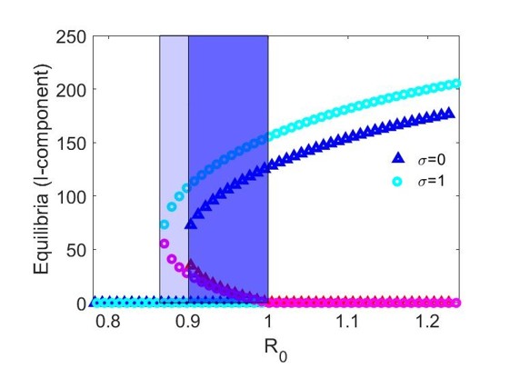
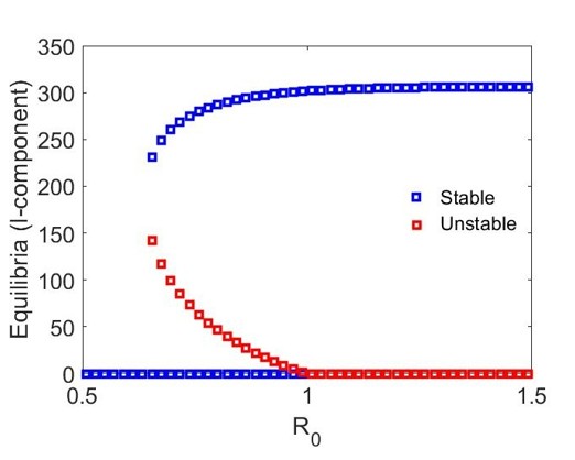
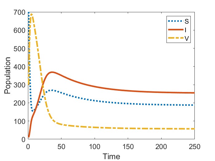
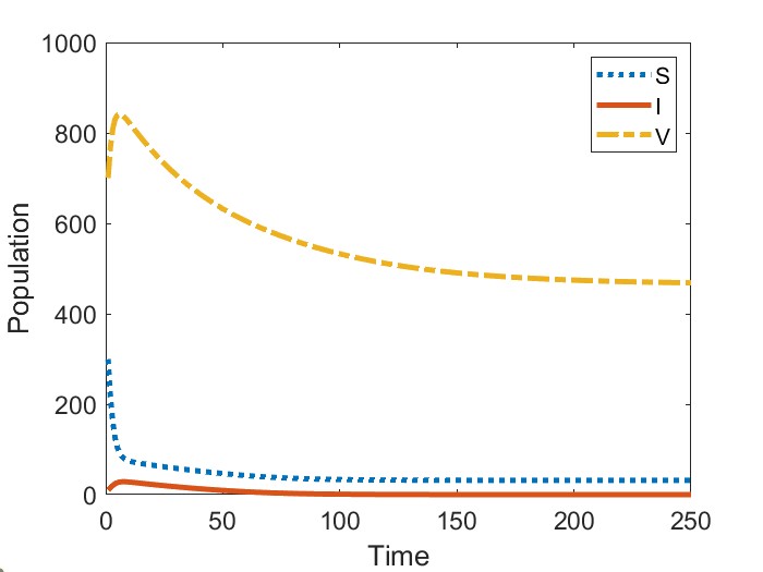
In Figure 2, we present the numerical results for the case when $ϵ=0.14$. Figure 2(a) gives the bifurcation diagram for the infected stage $I$ of model (1) using $R_0$ as the bifurcation parameter. As established in Theorem 2, the endemic equilibria bifurcating from $R_0=1$ are initially unstable. We observe that, in addition to this unstable branch, the model possesses a branch of stable endemic equilibria for $R_0>0.9$ when $\sigma =0$ and for $R_0>0.86$ when $\sigma =1$. As a result, for and , respectively, we observe bistable dynamics with both a stable disease-free equilibrium and a stable endemic equilibrium. In comparing the two cases, we observe that the range of $R_0$ values for which bistability occurs is larger when newly vaccinated individuals have the same risk of infection as previously vaccinated individuals ($\sigma =1$). Moreover, the asymptotic number of infectious individuals is also larger in this case.

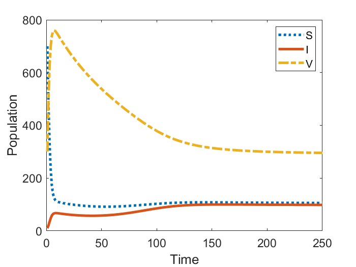
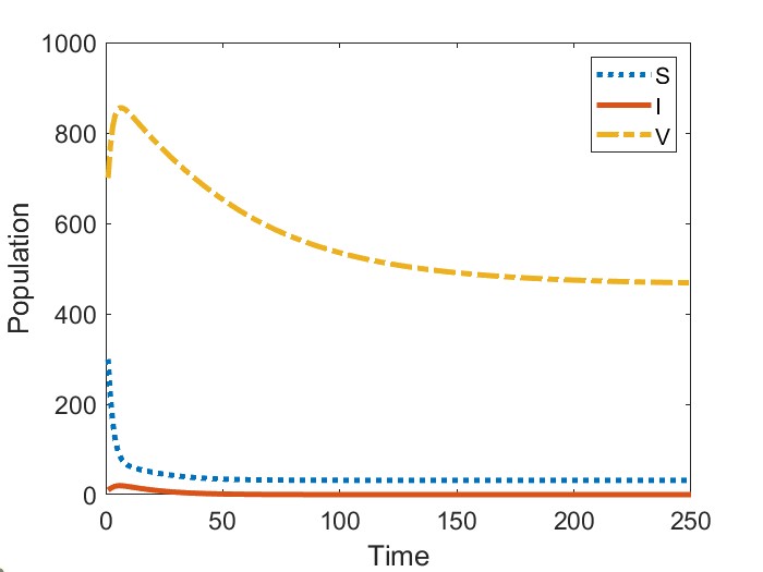
Figures 2(b)-2(c) give time series solutions for two different sets of initial conditions when $R_0=0.93$ ($\beta =3.3$) and $\sigma =0$ to illustrate this bistability. We observe that increasing the initial proportion of vaccinated individuals may lead to eradication of the disease.

(a)

(b)

(c)

Figure 2. (a) Shown is the bifurcation diagram for model (1) giving the asymptotic number of infected individual when $\sigma =0$ (triangles) and $\sigma =1$ (circles) when $ϵ=0.14$. Here unstable equilibria are given in red and magenta and stable equilibria are given in blue and cyan. (b)-(c) Time series solution of model (1) when $\sigma =0$ and $\beta =3.3$ with initial conditions (b) $S(0)=700,I(0)=10,V(0)=300$ or (c) $S(0)=300,I(0)=10,V(0)=700$. All graphs use the parameter values given in (15).

Example 5.2 (Influence of vaccination timing).

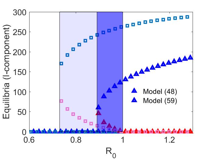
In this example, we consider the impact of timing of event assumptions by comparing vaccination before disease transmission to vaccination after disease transmission, as given by models (1) and (12), respectively. Using the parameter values given by (15), we find that condition (i) of Theorem 3 is satisfied. Thus, for model (12), there exists a branch of backward bifurcating equilibria at $R_0=1$, corresponding to $\beta =3.19$, for . In Figure 3 we compare the resulting backward bifurcations in the two models, using $\sigma =0$ for model (1). We observe that disease transmission before vaccination makes disease eradication more difficult, as the disease may persist for smaller $R_0$ values. It also results in a higher number of infected individuals whenever the infection does not die out.

Figure 3. Shown is the bifurcation diagram for models (1) (triangles) and (12) (squares), with $\sigma =0$, $ϵ=0.14$, and the remaining parameters values given by (15). Stable equilibria are given in blue and grey-blue and unstable are given in red and pink.

Finally, in Figure (4) we provide an example of a backward bifurcation in model (12) when vaccination is completely effective. For this figure, we keep all parameters the same except we set $ϵ=0$, resulting in a critical value of $\beta =9.74$. We again observe that sufficiently increasing the initial proportion of vaccinated individuals may eradicate the disease.

(a)

(b)

(c)

Figure 4. (a) Shown is the bifurcation diagram for model (12) giving the asymptotic number of infected individual with red rectangles denoting unstable equilibria and blue rectangles denoting stable equilibria. (b)-(c) The time series solution of model (12) when $\beta =9$, resulting in $R_0=0.94$, with initial conditions (b) $S(0)=700,I(0)=10,V(0)=300$ or (c) $S(0)=300,I(0)=10,V(0)=700$. All graphs use $ϵ=0$ with the remaining parameter values given in (15).

Example 5.3 (Multiple Attractors).

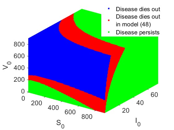
In this example, we examine the basins of attraction corresponding to the disease-free and endemic outcomes with respect to the initial conditions $(S_0,I_0,V_0)$ for models (1) and (12). Using the parameter values specified in (15), both models exhibit multiple attractors, namely, the disease-free equilibrium and the endemic equilibrium, within the bistability region when with corresponding $\beta =3.35$ and $\beta =3.02$ in model (1) and (12) respectively.

Our results show that for initial conditions $(S_0,I_0,V_0)$ located in the blue region, the solutions of both models converge to the disease-free equilibrium. In contrast, for initial conditions in the red region, only the solution of model (1) converges to the disease-free attractor. Finally, for initial conditions in the green region, both models converge to the endemic equilibrium. These observations indicate that model (1) has a larger area for disease elimination than model (12). As a result, we conclude that disease elimination is more difficult in model (12) than in model (1) in the bistable region.

Figure 5. Basins of attraction for the disease-free and endemic equilibria in model (1) and (12), where the blue, red, and green regions are, respectively, the basin of attraction of disease-free attractors for both models, disease-free attractor in model (1), and endemic attractor for both models.

6. Concluding Remarks

We developed two discrete-time SISV models to investigate how vaccination influences infection dynamics. In this framework, vaccination reduces the probability of infection but may not eliminate infection risk. For these models, we established a global stability result for the disease-free equilibrium and derived conditions for the existence of a backward bifurcation when the disease-free equilibrium destabilizes at $R_0=1$. This latter result used an extension of the Fundamental Bifurcation Theorem that was developed independently by the authors in [ackleh2023interplay] as well as in [elaydi2025discrete]. We remark that this model formulation differs from the discrete-time SISV model studied in [jang2008backward] in that it does not require assumptions on the size of the force of infection term to maintain positivity of solutions. In this previous work, the infection term in the model was given by the mass action form commonly used in continuous time, and thus, studying the endemic dynamics reduced to examining the solutions to a quadratic function. In contrast, when infection is described by the negative exponential term considered in Section 5 (a common assumption in discrete-time epidemic models), this becomes a much more challenging problem given that it is not possible to obtain explicit solutions for the endemic equilibria, thus making a bifurcation approach fitting for these models.

The two models presented in this paper differ in the order that vaccination and infection occur within a discrete time unit. By comparison, continuous-time models do not face this issue, as they assume events occur simultaneously. We found that the two model formulations present contrasting outcomes. Specifically, when vaccination occurs first, we showed that both infection recovery and partial vaccine efficiency are needed for a backward bifurcation to occur. This result is analogous to the findings for the continuous-time model formulation. However, if infection occurs before vaccination, we showed that it is possible for a backward bifurcation to occur even when the vaccine is fully effective. We also found that, when disease transmission occurs before vaccination, the region of bistablity is larger, implying that $R_0$ must be reduced even further to guarantee elimination of the disease. Moreover, the asymptotic number of infected individuals is larger in this bistability region, resulting in a more severe epidemic when the disease is not successfully eradicated. Similar behavior was observed in the first model (vaccination before infection) when comparing different infection rates in newly vaccinated individuals. Specifically, worse outcomes occur if the vaccine is not immediately effective.

These findings highlight the importance of early intervention strategies, as the results suggest that reducing the initial availability of susceptible individuals may mitigate the impact of the epidemic. The contrasting outcomes presented by the two models developed here bring up important questions as to what are the practical implications of these modeling assumptions? Specifically, in a real-world application, what does it mean to say that vaccination occurs before infection? In certain situations, such as examining the course of influenza throughout the year, this is clear: vaccination should ideally occur before the flu season begins. However, on a shorter timescale this distinction becomes less straightforward. We also note that another possible model formulation would be to assume that only one event, infection or vaccination, may occur within a unit of time. Under this assumption, it would be necessary to impose the additional assumption that $p+\varphi (z)\le 1$.

Since one of the goals of this paper was to determine whether the backward bifurcation that characterizes continuous-time SISV models with partial vaccination efficiency can also occur in a discrete-time, the models presented here were kept relatively simple. Consequently, a number of extensions could be considered, including disease-induced mortality, vaccination waning, and disease treatment, the latter of which may produce backward bifurcations in endemic equilibria (see for example [guerrero2018different, wang2009backward]). We also remark that, while we showed that a backward bifurcation cannot occur in model (1) when $ϵ=0$, we were unable to use the Lyapunov function developed in [van2019disease] to establish the global asymptotic stability of the disease-free equilibrium in this case. The difficulty arose because, unlike the case when there is no infection recovery ($\gamma =0$), the system does not decouple, making it challenging to show that the number of susceptible individuals is eventually bounded by the $S$-component of the disease-free equilibrium.